Learning Curve
Visualizer |
|
Quick Method |
|
Models |
Classification, Regression, Clustering |
Workflow |
Model Selection |
A learning curve shows the relationship of the training score versus the cross validated test score for an estimator with a varying number of training samples. This visualization is typically used to show two things:
How much the estimator benefits from more data (e.g. do we have “enough data” or will the estimator get better if used in an online fashion).
If the estimator is more sensitive to error due to variance vs. error due to bias.
Consider the following learning curves (generated with Yellowbrick, but from Plotting Learning Curves in the scikit-learn documentation):
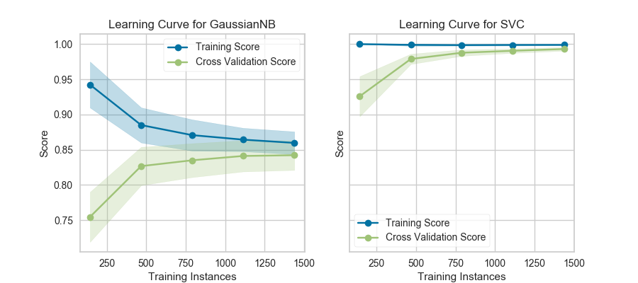
If the training and cross-validation scores converge together as more data is added (shown in the left figure), then the model will probably not benefit from more data. If the training score is much greater than the validation score then the model probably requires more training examples in order to generalize more effectively.
The curves are plotted with the mean scores, however variability during cross-validation is shown with the shaded areas that represent a standard deviation above and below the mean for all cross-validations. If the model suffers from error due to bias, then there will likely be more variability around the training score curve. If the model suffers from error due to variance, then there will be more variability around the cross validated score.
Note
Learning curves can be generated for all estimators that have fit() and predict() methods as well as a single scoring metric. This includes classifiers, regressors, and clustering as we will see in the following examples.
Classification
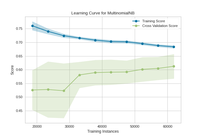
In the following example, we show how to visualize the learning curve of a classification model. After loading a DataFrame and performing categorical encoding, we create a StratifiedKFold cross-validation strategy to ensure all of our classes in each split are represented with the same proportion. We then fit the visualizer using the f1_weighted scoring metric as opposed to the default metric, accuracy, to get a better sense of the relationship of precision and recall in our classifier.
import numpy as np

from sklearn.model_selection import StratifiedKFold
from sklearn.naive_bayes import MultinomialNB
from sklearn.preprocessing import OneHotEncoder, LabelEncoder

from yellowbrick.datasets import load_game
from yellowbrick.model_selection import LearningCurve

# Load a classification dataset
X, y = load_game()

# Encode the categorical data
X = OneHotEncoder().fit_transform(X)
y = LabelEncoder().fit_transform(y)

# Create the learning curve visualizer
cv = StratifiedKFold(n_splits=12)
sizes = np.linspace(0.3, 1.0, 10)

# Instantiate the classification model and visualizer
model = MultinomialNB()
visualizer = LearningCurve(
    model, cv=cv, scoring='f1_weighted', train_sizes=sizes, n_jobs=4
)

visualizer.fit(X, y)        # Fit the data to the visualizer
visualizer.show()           # Finalize and render the figure
(Source code, png, pdf)

This learning curve shows high test variability and a low score up to around 30,000 instances, however after this level the model begins to converge on an F1 score of around 0.6. We can see that the training and test scores have not yet converged, so potentially this model would benefit from more training data. Finally, this model suffers primarily from error due to variance (the CV scores for the test data are more variable than for training data) so it is possible that the model is overfitting.
Regression
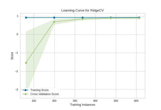
Building a learning curve for a regression is straight forward and very similar. In the below example, after loading our data and selecting our target, we explore the learning curve score according to the coefficient of determination or R2 score.
from sklearn.linear_model import RidgeCV

from yellowbrick.datasets import load_energy
from yellowbrick.model_selection import LearningCurve

# Load a regression dataset
X, y = load_energy()

# Instantiate the regression model and visualizer
model = RidgeCV()
visualizer = LearningCurve(model, scoring='r2')

visualizer.fit(X, y)        # Fit the data to the visualizer
visualizer.show()           # Finalize and render the figure
(Source code, png, pdf)

This learning curve shows a very high variability and much lower score until about 350 instances. It is clear that this model could benefit from more data because it is converging at a very high score. Potentially, with more data and a larger alpha for regularization, this model would become far less variable in the test data.
Clustering
Learning curves also work for clustering models and can use metrics that specify the shape or organization of clusters such as silhouette scores or density scores. If the membership is known in advance, then rand scores can be used to compare clustering performance as shown below:
from sklearn.cluster import KMeans
from sklearn.datasets import make_blobs

from yellowbrick.model_selection import LearningCurve

# Generate synthetic dataset with 5 random clusters
X, y = make_blobs(n_samples=1000, centers=5, random_state=42)

# Instantiate the clustering model and visualizer
model = KMeans()
visualizer = LearningCurve(model, scoring="adjusted_rand_score", random_state=42)

visualizer.fit(X, y)        # Fit the data to the visualizer
visualizer.show()           # Finalize and render the figure
(Source code, png, pdf)
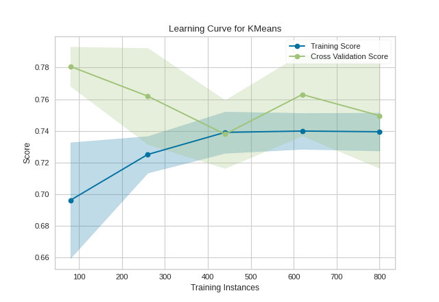
Unfortunately, with random data these curves are highly variable, but serve to point out some clustering-specific items. First, note the y-axis is very narrow, roughly speaking these curves are converged and actually the clustering algorithm is performing very well. Second, for clustering, convergence for data points is not necessarily a bad thing; in fact we want to ensure as more data is added, the training and cross-validation scores do not diverge.
Quick Method
The same functionality can be achieved with the associated quick method learning_curve. This method will build the LearningCurve object with the associated arguments, fit it, then (optionally) immediately show the visualization.
from sklearn.linear_model import RidgeCV

from yellowbrick.datasets import load_energy
from yellowbrick.model_selection import learning_curve

# Load a regression dataset
X, y = load_energy()

learning_curve(RidgeCV(), X, y, scoring='r2')
(Source code, png, pdf)
See also
This visualizer is based on the validation curve described in the scikit-learn documentation: Learning Curves. The visualizer wraps the learning_curve function and most of the arguments are passed directly to it.
API Reference
Implements a learning curve visualization for model selection.
- class yellowbrick.model_selection.learning_curve.LearningCurve(estimator, ax=None, groups=None, train_sizes=array([0.1, 0.325, 0.55, 0.775, 1.0]), cv=None, scoring=None, exploit_incremental_learning=False, n_jobs=1, pre_dispatch='all', shuffle=False, random_state=None, **kwargs)[source]
Bases:
ModelVisualizerVisualizes the learning curve for both test and training data for different training set sizes. These curves can act as a proxy to demonstrate the implied learning rate with experience (e.g. how much data is required to make an adequate model). They also demonstrate if the model is more sensitive to error due to bias vs. error due to variance and can be used to quickly check if a model is overfitting.
The visualizer evaluates cross-validated training and test scores for different training set sizes. These curves are plotted so that the x-axis is the training set size and the y-axis is the score.
The cross-validation generator splits the whole dataset k times, scores are averaged over all k runs for the training subset. The curve plots the mean score for the k splits, and the filled in area suggests the variability of the cross-validation by plotting one standard deviation above and below the mean for each split.
- Parameters
- estimatora scikit-learn estimator
An object that implements
fitandpredict, can be a classifier, regressor, or clusterer so long as there is also a valid associated scoring metric.Note that the object is cloned for each validation.
- axmatplotlib.Axes object, optional
The axes object to plot the figure on.
- groupsarray-like, with shape (n_samples,)
Optional group labels for the samples used while splitting the dataset into train/test sets.
- train_sizesarray-like, shape (n_ticks,)
default:
np.linspace(0.1,1.0,5)Relative or absolute numbers of training examples that will be used to generate the learning curve. If the dtype is float, it is regarded as a fraction of the maximum size of the training set, otherwise it is interpreted as absolute sizes of the training sets.
- cvint, cross-validation generator or an iterable, optional
Determines the cross-validation splitting strategy. Possible inputs for cv are:
None, to use the default 3-fold cross-validation,
integer, to specify the number of folds.
An object to be used as a cross-validation generator.
An iterable yielding train/test splits.
see the scikit-learn cross-validation guide for more information on the possible strategies that can be used here.
- scoringstring, callable or None, optional, default: None
A string or scorer callable object / function with signature
scorer(estimator, X, y). See scikit-learn model evaluation documentation for names of possible metrics.- exploit_incremental_learningboolean, default: False
If the estimator supports incremental learning, this will be used to speed up fitting for different training set sizes.
- n_jobsinteger, optional
Number of jobs to run in parallel (default 1).
- pre_dispatchinteger or string, optional
Number of predispatched jobs for parallel execution (default is all). The option can reduce the allocated memory. The string can be an expression like ‘2*n_jobs’.
- shuffleboolean, optional
Whether to shuffle training data before taking prefixes of it based on``train_sizes``.
- random_stateint, RandomState instance or None, optional (default=None)
If int, random_state is the seed used by the random number generator; If RandomState instance, random_state is the random number generator; If None, the random number generator is the RandomState instance used by np.random. Used when
shuffleis True.- kwargsdict
Keyword arguments that are passed to the base class and may influence the visualization as defined in other Visualizers.
Notes
This visualizer is essentially a wrapper for the
sklearn.model_selection.learning_curve utility, discussed in the validation curves documentation.See also
The documentation for the learning_curve function, which this visualizer wraps.
Examples
>>> from yellowbrick.model_selection import LearningCurve
>>> from sklearn.naive_bayes import GaussianNB
>>> model = LearningCurve(GaussianNB())
>>> model.fit(X, y)
>>> model.show()
- Attributes
- train_sizes_array, shape = (n_unique_ticks,), dtype int
Numbers of training examples that has been used to generate the learning curve. Note that the number of ticks might be less than n_ticks because duplicate entries will be removed.
- train_scores_array, shape (n_ticks, n_cv_folds)
Scores on training sets.
- train_scores_mean_array, shape (n_ticks,)
Mean training data scores for each training split
- train_scores_std_array, shape (n_ticks,)
Standard deviation of training data scores for each training split
- test_scores_array, shape (n_ticks, n_cv_folds)
Scores on test set.
- test_scores_mean_array, shape (n_ticks,)
Mean test data scores for each test split
- test_scores_std_array, shape (n_ticks,)
Standard deviation of test data scores for each test split
- fit(X, y=None)[source]
Fits the learning curve with the wrapped model to the specified data. Draws training and test score curves and saves the scores to the estimator.
- Parameters
- Xarray-like, shape (n_samples, n_features)
Training vector, where n_samples is the number of samples and n_features is the number of features.
- yarray-like, shape (n_samples) or (n_samples, n_features), optional
Target relative to X for classification or regression; None for unsupervised learning.
- Returns
- selfinstance
Returns the instance of the learning curve visualizer for use in pipelines and other sequential transformers.
- yellowbrick.model_selection.learning_curve.learning_curve(estimator, X, y, ax=None, groups=None, train_sizes=array([0.1, 0.325, 0.55, 0.775, 1.0]), cv=None, scoring=None, exploit_incremental_learning=False, n_jobs=1, pre_dispatch='all', shuffle=False, random_state=None, show=True, **kwargs)[source]
Displays a learning curve based on number of samples vs training and cross validation scores. The learning curve aims to show how a model learns and improves with experience.
This helper function is a quick wrapper to utilize the LearningCurve for one-off analysis.
- Parameters
- estimatora scikit-learn estimator
An object that implements
fitandpredict, can be a classifier, regressor, or clusterer so long as there is also a valid associated scoring metric.Note that the object is cloned for each validation.
- Xarray-like, shape (n_samples, n_features)
Training vector, where n_samples is the number of samples and n_features is the number of features.
- yarray-like, shape (n_samples) or (n_samples, n_features), optional
Target relative to X for classification or regression; None for unsupervised learning.
- axmatplotlib.Axes object, optional
The axes object to plot the figure on.
- groupsarray-like, with shape (n_samples,)
Optional group labels for the samples used while splitting the dataset into train/test sets.
- train_sizesarray-like, shape (n_ticks,)
default:
np.linspace(0.1,1.0,5)Relative or absolute numbers of training examples that will be used to generate the learning curve. If the dtype is float, it is regarded as a fraction of the maximum size of the training set, otherwise it is interpreted as absolute sizes of the training sets.
- cvint, cross-validation generator or an iterable, optional
Determines the cross-validation splitting strategy. Possible inputs for cv are:
None, to use the default 3-fold cross-validation,
integer, to specify the number of folds.
An object to be used as a cross-validation generator.
An iterable yielding train/test splits.
see the scikit-learn cross-validation guide for more information on the possible strategies that can be used here.
- scoringstring, callable or None, optional, default: None
A string or scorer callable object / function with signature
scorer(estimator, X, y). See scikit-learn model evaluation documentation for names of possible metrics.- exploit_incremental_learningboolean, default: False
If the estimator supports incremental learning, this will be used to speed up fitting for different training set sizes.
- n_jobsinteger, optional
Number of jobs to run in parallel (default 1).
- pre_dispatchinteger or string, optional
Number of predispatched jobs for parallel execution (default is all). The option can reduce the allocated memory. The string can be an expression like ‘2*n_jobs’.
- shuffleboolean, optional
Whether to shuffle training data before taking prefixes of it based on``train_sizes``.
- random_stateint, RandomState instance or None, optional (default=None)
If int, random_state is the seed used by the random number generator; If RandomState instance, random_state is the random number generator; If None, the random number generator is the RandomState instance used by np.random. Used when
shuffleis True.- showbool, default: True
If True, calls
show(), which in turn callsplt.show()however you cannot callplt.savefigfrom this signature, norclear_figure. If False, simply callsfinalize()- kwargsdict
Keyword arguments that are passed to the base class and may influence the visualization as defined in other Visualizers. These arguments are also passed to the show() method, e.g. can pass a path to save the figure to.
- Returns
- visualizerLearningCurve
Returns the fitted visualizer.