Alpha Selection

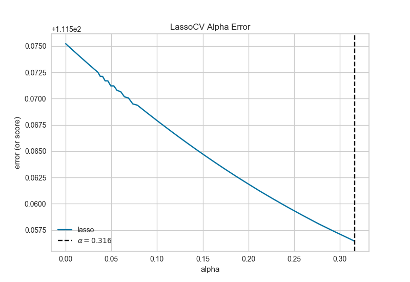
Regularization is designed to penalize model complexity, therefore the higher the alpha, the less complex the model, decreasing the error due to variance (overfit). Alphas that are too high on the other hand increase the error due to bias (underfit). It is important, therefore to choose an optimal alpha such that the error is minimized in both directions.

The AlphaSelection Visualizer demonstrates how different values of alpha influence model selection during the regularization of linear models. Generally speaking, alpha increases the affect of regularization, e.g. if alpha is zero there is no regularization and the higher the alpha, the more the regularization parameter influences the final model.

# Load the data
df = load_data('concrete')
feature_names = ['cement', 'slag', 'ash', 'water', 'splast', 'coarse', 'fine', 'age']
target_name = 'strength'

# Get the X and y data from the DataFrame
X = df[feature_names].as_matrix()
y = df[target_name].as_matrix()

# Create the train and test data
X_train, X_test, y_train, y_test = train_test_split(X, y, test_size=0.2)

# Create a list of alphas to cross-validate against
alphas = np.logspace(-12, -0.5, 400)

# Instantiate the linear model and visualizer
model = LassoCV(alphas=alphas)
visualizer = AlphaSelection(model)

visualizer.fit(X_train, y_train)  # Fit the training data to the visualizer
g = visualizer.poof()             # Draw/show/poof the data

API Reference

Implements alpha selection visualizers for regularization

class yellowbrick.regressor.alphas.AlphaSelection(model, ax=None, **kwargs)

基类：yellowbrick.regressor.base.RegressionScoreVisualizer

The Alpha Selection Visualizer demonstrates how different values of alpha influence model selection during the regularization of linear models. Generally speaking, alpha increases the affect of regularization, e.g. if alpha is zero there is no regularization and the higher the alpha, the more the regularization parameter influences the final model.

Regularization is designed to penalize model complexity, therefore the higher the alpha, the less complex the model, decreasing the error due to variance (overfit). Alphas that are too high on the other hand increase the error due to bias (underfit). It is important, therefore to choose an optimal Alpha such that the error is minimized in both directions.

To do this, typically you would you use one of the "RegressionCV" models in Scikit-Learn. E.g. instead of using the Ridge (L2) regularizer, you can use RidgeCV and pass a list of alphas, which will be selected based on the cross-validation score of each alpha. This visualizer wraps a "RegressionCV" model and visualizes the alpha/error curve. Use this visualization to detect if the model is responding to regularization, e.g. as you increase or decrease alpha, the model responds and error is decreased. If the visualization shows a jagged or random plot, then potentially the model is not sensitive to that type of regularization and another is required (e.g. L1 or Lasso regularization).

Parameters:

model : a Scikit-Learn regressor

Should be an instance of a regressor, and specifically one whose name ends with "CV" otherwise a will raise a YellowbrickTypeError exception on instantiation. To use non-CV regressors see: ManualAlphaSelection.

ax : matplotlib Axes, default: None

The axes to plot the figure on. If None is passed in the current axes will be used (or generated if required).

kwargs : dict

Keyword arguments that are passed to the base class and may influence the visualization as defined in other Visualizers.

Notes

This class expects an estimator whose name ends with "CV". If you wish to use some other estimator, please see the ManualAlphaSelection Visualizer for manually iterating through all alphas and selecting the best one.

This Visualizer hoooks into the Scikit-Learn API during fit(). In order to pass a fitted model to the Visualizer, call the draw() method directly after instantiating the visualizer with the fitted model.

Note, each "RegressorCV" module has many different methods for storing alphas and error. This visualizer attempts to get them all and is known to work for RidgeCV, LassoCV, LassoLarsCV, and ElasticNetCV. If your favorite regularization method doesn't work, please submit a bug report.

For RidgeCV, make sure store_cv_values=True.

Examples

>>> from yellowbrick.regressor import AlphaSelection
>>> from sklearn.linear_model import LassoCV
>>> model = AlphaSelection(LassoCV())
>>> model.fit(X, y)
>>> model.poof()

draw()

Draws the alpha plot based on the values on the estimator.

finalize()

Prepare the figure for rendering by setting the title as well as the X and Y axis labels and adding the legend.

fit(X, y, **kwargs)

A simple pass-through method; calls fit on the estimator and then draws the alpha-error plot.

class yellowbrick.regressor.alphas.ManualAlphaSelection(model, ax=None, alphas=None, cv=None, scoring=None, **kwargs)

基类：yellowbrick.regressor.alphas.AlphaSelection

The AlphaSelection visualizer requires a "RegressorCV", that is a specialized class that performs cross-validated alpha-selection on behalf of the model. If the regressor you wish to use doesn't have an associated "CV" estimator, or for some reason you would like to specify more control over the alpha selection process, then you can use this manual alpha selection visualizer, which is essentially a wrapper for cross_val_score, fitting a model for each alpha specified.

Parameters:

model : a Scikit-Learn regressor

Should be an instance of a regressor, and specifically one whose name doesn't end with "CV". The regressor must support a call to set_params(alpha=alpha) and be fit multiple times. If the regressor name ends with "CV" a YellowbrickValueError is raised.

ax : matplotlib Axes, default: None

The axes to plot the figure on. If None is passed in the current axes will be used (or generated if required).

alphas : ndarray or Series, default: np.logspace(-10, 2, 200)

An array of alphas to fit each model with

cv : int, cross-validation generator or an iterable, optional

Determines the cross-validation splitting strategy. Possible inputs for cv are:

• None, to use the default 3-fold cross validation,
• integer, to specify the number of folds in a (Stratified)KFold,
• An object to be used as a cross-validation generator.
• An iterable yielding train, test splits.

This argument is passed to the sklearn.model_selection.cross_val_score method to produce the cross validated score for each alpha.

scoring : string, callable or None, optional, default: None

A string (see model evaluation documentation) or a scorer callable object / function with signature scorer(estimator, X, y).

This argument is passed to the sklearn.model_selection.cross_val_score method to produce the cross validated score for each alpha.

kwargs : dict

Keyword arguments that are passed to the base class and may influence the visualization as defined in other Visualizers.

Notes

This class does not take advantage of estimator-specific searching and is therefore less optimal and more time consuming than the regular "RegressorCV" estimators.

Examples

>>> from yellowbrick.regressor import ManualAlphaSelection
>>> from sklearn.linear_model import Ridge
>>> model = ManualAlphaSelection(
...     Ridge(), cv=12, scoring='neg_mean_squared_error'
... )
...
>>> model.fit(X, y)
>>> model.poof()

draw()

Draws the alphas values against their associated error in a similar fashion to the AlphaSelection visualizer.

fit(X, y, **args)

The fit method is the primary entry point for the manual alpha selection visualizer. It sets the alpha param for each alpha in the alphas list on the wrapped estimator, then scores the model using the passed in X and y data set. Those scores are then aggregated and drawn using matplotlib.