Validation Curve
Model validation is used to determine how effective an estimator is on data that it has been trained on as well as how generalizable it is to new input. To measure a model’s performance we first split the dataset into training and test splits, fitting the model on the training data and scoring it on the reserved test data.
In order to maximize the score, the hyperparameters of the model must be selected which best allow the model to operate in the specified feature space. Most models have multiple hyperparameters and the best way to choose a combination of those parameters is with a grid search. However, it is sometimes useful to plot the influence of a single hyperparameter on the training and test data to determine if the estimator is underfitting or overfitting for some hyperparameter values.
Visualizer |
|
Quick Method |
|
Models |
Classification and Regression |
Workflow |
Model Selection |
In our first example, we’ll explore using the ValidationCurve visualizer with a regression dataset and in the second, a classification dataset. Note that any estimator that implements fit() and predict() and has an appropriate scoring mechanism can be used with this visualizer.
import numpy as np

from yellowbrick.datasets import load_energy
from yellowbrick.model_selection import ValidationCurve

from sklearn.tree import DecisionTreeRegressor

# Load a regression dataset
X, y = load_energy()

viz = ValidationCurve(
    DecisionTreeRegressor(), param_name="max_depth",
    param_range=np.arange(1, 11), cv=10, scoring="r2"
)

# Fit and show the visualizer
viz.fit(X, y)
viz.show()
(Source code, png, pdf)

To further customize this plot, the visualizer also supports a markers parameter that changes the marker style.
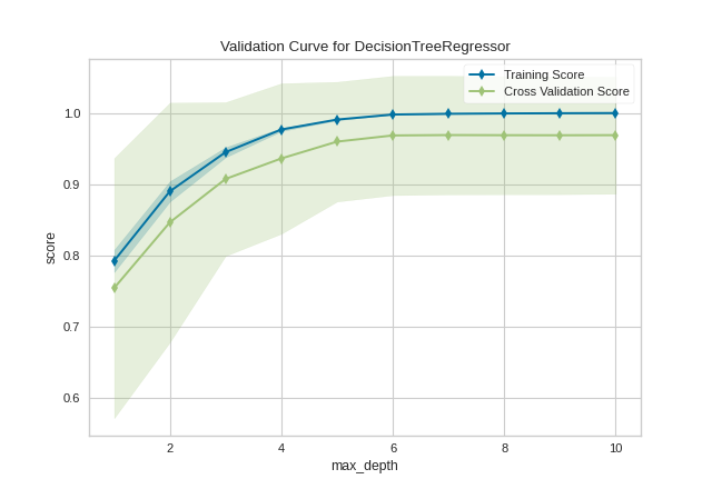
After loading and wrangling the data, we initialize the ValidationCurve with a DecisionTreeRegressor. Decision trees become more overfit the deeper they are because at each level of the tree the partitions are dealing with a smaller subset of data. One way to deal with this overfitting process is to limit the depth of the tree. The validation curve explores the relationship of the "max_depth" parameter to the R2 score with 10 shuffle split cross-validation. The param_range argument specifies the values of max_depth, here from 1 to 10 inclusive.
We can see in the resulting visualization that a depth limit of less than 5 levels severely underfits the model on this data set because the training score and testing score climb together in this parameter range, and because of the high variability of cross validation on the test scores. After a depth of 7, the training and test scores diverge, this is because deeper trees are beginning to overfit the training data, providing no generalizability to the model. However, because the cross validation score does not necessarily decrease, the model is not suffering from high error due to variance.
In the next visualizer, we will see an example that more dramatically visualizes the bias/variance tradeoff.
from sklearn.svm import SVC
from sklearn.preprocessing import OneHotEncoder
from sklearn.model_selection import StratifiedKFold

# Load a classification data set
X, y = load_game()

# Encode the categorical data with one-hot encoding
X = OneHotEncoder().fit_transform(X)

# Create the validation curve visualizer
cv = StratifiedKFold(12)
param_range = np.logspace(-6, -1, 12)

viz = ValidationCurve(
    SVC(), param_name="gamma", param_range=param_range,
    logx=True, cv=cv, scoring="f1_weighted", n_jobs=8,
)

viz.fit(X, y)
viz.show()
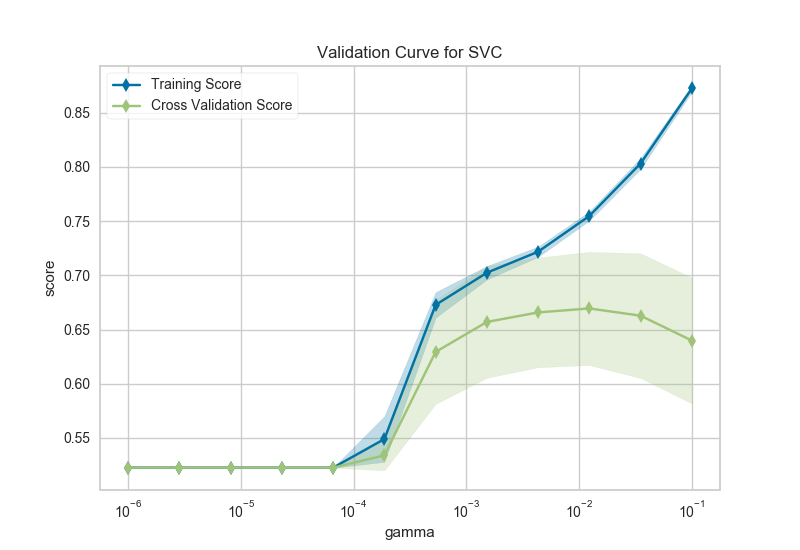
After loading data and one-hot encoding it using the Pandas get_dummies function, we create a stratified k-folds cross-validation strategy. The hyperparameter of interest is the gamma of a support vector classifier, the coefficient of the RBF kernel. Gamma controls how much influence a single example has, the larger gamma is, the tighter the support vector is around single points (overfitting the model).
In this visualization we see a definite inflection point around gamma=0.1. At this point the training score climbs rapidly as the SVC memorizes the data, while the cross-validation score begins to decrease as the model cannot generalize to unseen data.
Warning
Note that running this and the next example may take a long time. Even with parallelism using n_jobs=8, it can take several hours to go through all the combinations. Reducing the parameter range and minimizing the amount of cross-validation can speed up the validation curve visualization.
Validation curves can be performance intensive since they are training n_params * n_splits models and scoring them. It is critically important to ensure that the specified hyperparameter range is correct, as we will see in the next example.
from sklearn.neighbors import KNeighborsClassifier

cv = StratifiedKFold(4)
param_range = np.arange(3, 20, 2)

oz = ValidationCurve(
    KNeighborsClassifier(), param_name="n_neighbors",
    param_range=param_range, cv=cv, scoring="f1_weighted", n_jobs=4,
)

# Using the same game dataset as in the SVC example
oz.fit(X, y)
oz.show()
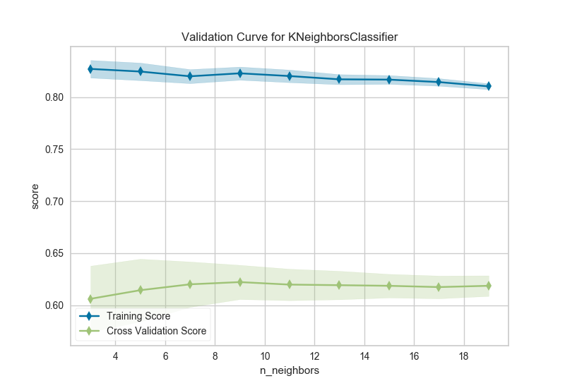
The k nearest neighbors (kNN) model is commonly used when similarity is important to the interpretation of the model. Choosing k is difficult, the higher k is the more data is included in a classification, creating more complex decision topologies, whereas the lower k is, the simpler the model is and the less it may generalize. Using a validation curve seems like an excellent strategy for choosing k, and often it is. However in the example above, all we can see is a decreasing variability in the cross-validated scores.
This validation curve poses two possibilities: first, that we do not have the correct param_range to find the best k and need to expand our search to larger values. The second is that other hyperparameters (such as uniform or distance based weighting, or even the distance metric) may have more influence on the default model than k by itself does. Although validation curves can give us some intuition about the performance of a model to a single hyperparameter, grid search is required to understand the performance of a model with respect to multiple hyperparameters.
See also
This visualizer is based on the validation curve described in the scikit-learn documentation: Validation Curves. The visualizer wraps the validation_curve function and most of the arguments are passed directly to it.
Quick Method
Similar functionality as above can be achieved in one line using the associated quick method, validation_curve. This method will instantiate and fit a ValidationCurve visualizer.
import numpy as np

from yellowbrick.datasets import load_energy
from yellowbrick.model_selection import validation_curve

from sklearn.tree import DecisionTreeRegressor

# Load a regression dataset
X, y = load_energy()

viz = validation_curve(
    DecisionTreeRegressor(), X, y, param_name="max_depth",
    param_range=np.arange(1, 11), cv=10, scoring="r2",
)
(Source code, png, pdf)

API Reference
Implements a visual validation curve for a hyperparameter.
- class yellowbrick.model_selection.validation_curve.ValidationCurve(estimator, param_name, param_range, ax=None, logx=False, groups=None, cv=None, scoring=None, n_jobs=1, pre_dispatch='all', markers='-d', **kwargs)[source]
Bases:
ModelVisualizerVisualizes the validation curve for both test and training data for a range of values for a single hyperparameter of the model. Adjusting the value of a hyperparameter adjusts the complexity of a model. Less complex models suffer from increased error due to bias, while more complex models suffer from increased error due to variance. By inspecting the training and cross-validated test score error, it is possible to estimate a good value for a hyperparameter that balances the bias/variance trade-off.
The visualizer evaluates cross-validated training and test scores for the different hyperparameters supplied. The curve is plotted so that the x-axis is the value of the hyperparameter and the y-axis is the model score. This is similar to a grid search with a single hyperparameter.
The cross-validation generator splits the dataset k times, and scores are averaged over all k runs for the training and test subsets. The curve plots the mean score, and the filled in area suggests the variability of cross-validation by plotting one standard deviation above and below the mean for each split.
- Parameters
- estimatora scikit-learn estimator
An object that implements
fitandpredict, can be a classifier, regressor, or clusterer so long as there is also a valid associated scoring metric.Note that the object is cloned for each validation.
- param_namestring
Name of the parameter that will be varied.
- param_rangearray-like, shape (n_values,)
The values of the parameter that will be evaluated.
- axmatplotlib.Axes object, optional
The axes object to plot the figure on.
- logxboolean, optional
If True, plots the x-axis with a logarithmic scale.
- groupsarray-like, with shape (n_samples,)
Optional group labels for the samples used while splitting the dataset into train/test sets.
- cvint, cross-validation generator or an iterable, optional
Determines the cross-validation splitting strategy. Possible inputs for cv are:
None, to use the default 3-fold cross-validation,
integer, to specify the number of folds.
An object to be used as a cross-validation generator.
An iterable yielding train/test splits.
see the scikit-learn cross-validation guide for more information on the possible strategies that can be used here.
- scoringstring, callable or None, optional, default: None
A string or scorer callable object / function with signature
scorer(estimator, X, y). See scikit-learn model evaluation documentation for names of possible metrics.- n_jobsinteger, optional
Number of jobs to run in parallel (default 1).
- pre_dispatchinteger or string, optional
Number of predispatched jobs for parallel execution (default is all). The option can reduce the allocated memory. The string can be an expression like ‘2*n_jobs’.
- markersstring, default: ‘-d’
Matplotlib style markers for points on the plot points Options: ‘-,’, ‘-+’, ‘-o’, ‘-*’, ‘-v’, ‘-h’, ‘-d’
- kwargsdict
Keyword arguments that are passed to the base class and may influence the visualization as defined in other Visualizers.
Notes
This visualizer is essentially a wrapper for the
sklearn.model_selection.learning_curve utility, discussed in the validation curves documentation.See also
The documentation for the learning_curve function, which this visualizer wraps.
Examples
>>> import numpy as np
>>> from yellowbrick.model_selection import ValidationCurve
>>> from sklearn.svm import SVC
>>> pr = np.logspace(-6,-1,5)
>>> model = ValidationCurve(SVC(), param_name="gamma", param_range=pr)
>>> model.fit(X, y)
>>> model.show()
- Attributes
- train_scores_array, shape (n_ticks, n_cv_folds)
Scores on training sets.
- train_scores_mean_array, shape (n_ticks,)
Mean training data scores for each training split
- train_scores_std_array, shape (n_ticks,)
Standard deviation of training data scores for each training split
- test_scores_array, shape (n_ticks, n_cv_folds)
Scores on test set.
- test_scores_mean_array, shape (n_ticks,)
Mean test data scores for each test split
- test_scores_std_array, shape (n_ticks,)
Standard deviation of test data scores for each test split
- fit(X, y=None)[source]
Fits the validation curve with the wrapped estimator and parameter array to the specified data. Draws training and test score curves and saves the scores to the visualizer.
- Parameters
- Xarray-like, shape (n_samples, n_features)
Training vector, where n_samples is the number of samples and n_features is the number of features.
- yarray-like, shape (n_samples) or (n_samples, n_features), optional
Target relative to X for classification or regression; None for unsupervised learning.
- Returns
- selfinstance
Returns the instance of the validation curve visualizer for use in pipelines and other sequential transformers.
- yellowbrick.model_selection.validation_curve.validation_curve(estimator, X, y, param_name, param_range, ax=None, logx=False, groups=None, cv=None, scoring=None, n_jobs=1, pre_dispatch='all', show=True, markers='-d', **kwargs)[source]
Displays a validation curve for the specified param and values, plotting both the train and cross-validated test scores. The validation curve is a visual, single-parameter grid search used to tune a model to find the best balance between error due to bias and error due to variance.
This helper function is a wrapper to use the ValidationCurve in a fast, visual analysis.
- Parameters
- estimatora scikit-learn estimator
An object that implements
fitandpredict, can be a classifier, regressor, or clusterer so long as there is also a valid associated scoring metric.Note that the object is cloned for each validation.
- Xarray-like, shape (n_samples, n_features)
Training vector, where n_samples is the number of samples and n_features is the number of features.
- yarray-like, shape (n_samples) or (n_samples, n_features), optional
Target relative to X for classification or regression; None for unsupervised learning.
- param_namestring
Name of the parameter that will be varied.
- param_rangearray-like, shape (n_values,)
The values of the parameter that will be evaluated.
- axmatplotlib.Axes object, optional
The axes object to plot the figure on.
- logxboolean, optional
If True, plots the x-axis with a logarithmic scale.
- groupsarray-like, with shape (n_samples,)
Optional group labels for the samples used while splitting the dataset into train/test sets.
- cvint, cross-validation generator or an iterable, optional
Determines the cross-validation splitting strategy. Possible inputs for cv are:
None, to use the default 3-fold cross-validation,
integer, to specify the number of folds.
An object to be used as a cross-validation generator.
An iterable yielding train/test splits.
see the scikit-learn cross-validation guide for more information on the possible strategies that can be used here.
- scoringstring, callable or None, optional, default: None
A string or scorer callable object / function with signature
scorer(estimator, X, y). See scikit-learn model evaluation documentation for names of possible metrics.- n_jobsinteger, optional
Number of jobs to run in parallel (default 1).
- pre_dispatchinteger or string, optional
Number of predispatched jobs for parallel execution (default is all). The option can reduce the allocated memory. The string can be an expression like ‘2*n_jobs’.
- show: bool, default: True
If True, calls
show(), which in turn callsplt.show()however you cannot callplt.savefigfrom this signature, norclear_figure. If False, simply callsfinalize()- markersstring, default: ‘-d’
Matplotlib style markers for points on the plot points Options: ‘-,’, ‘-+’, ‘-o’, ‘-*’, ‘-v’, ‘-h’, ‘-d’
- kwargsdict
Keyword arguments that are passed to the base class and may influence the visualization as defined in other Visualizers. These arguments are also passed to the
show()method, e.g. can pass a path to save the figure to.
- Returns
- visualizerValidationCurve
The fitted visualizer