Discrimination Threshold
Caution
This visualizer only works for binary classification.
A visualization of precision, recall, f1 score, and queue rate with respect to the discrimination threshold of a binary classifier. The discrimination threshold is the probability or score at which the positive class is chosen over the negative class. Generally, this is set to 50% but the threshold can be adjusted to increase or decrease the sensitivity to false positives or to other application factors.
Visualizer |
|
Quick Method |
|
Models |
Classification |
Workflow |
Model evaluation |
from sklearn.linear_model import LogisticRegression

from yellowbrick.classifier import DiscriminationThreshold
from yellowbrick.datasets import load_spam

# Load a binary classification dataset
X, y = load_spam()

# Instantiate the classification model and visualizer
model = LogisticRegression(multi_class="auto", solver="liblinear")
visualizer = DiscriminationThreshold(model)

visualizer.fit(X, y)        # Fit the data to the visualizer
visualizer.show()           # Finalize and render the figure
(Source code, png, pdf)
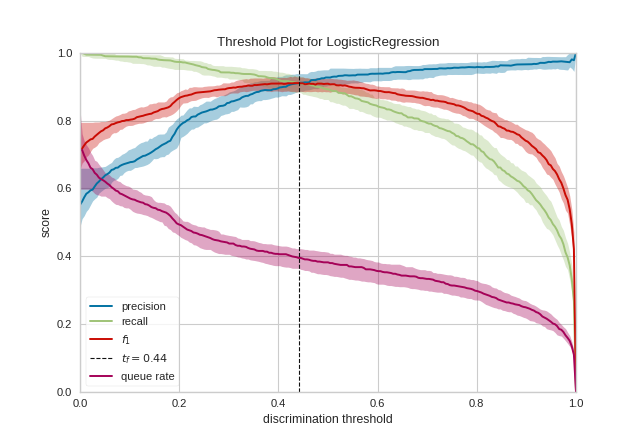
One common use of binary classification algorithms is to use the score or probability they produce to determine cases that require special treatment. For example, a fraud prevention application might use a classification algorithm to determine if a transaction is likely fraudulent and needs to be investigated in detail. In the figure above, we present an example where a binary classifier determines if an email is “spam” (the positive case) or “not spam” (the negative case). Emails that are detected as spam are moved to a hidden folder and eventually deleted.
Many classifiers use either a decision_function to score the positive class or a predict_proba function to compute the probability of the positive class. If the score or probability is greater than some discrimination threshold then the positive class is selected, otherwise, the negative class is.
Generally speaking, the threshold is balanced between cases and set to 0.5 or 50% probability. However, this threshold may not be the optimal threshold: often there is an inverse relationship between precision and recall with respect to a discrimination threshold. By adjusting the threshold of the classifier, it is possible to tune the F1 score (the harmonic mean of precision and recall) to the best possible fit or to adjust the classifier to behave optimally for the specific application. Classifiers are tuned by considering the following metrics:
Precision: An increase in precision is a reduction in the number of false positives; this metric should be optimized when the cost of special treatment is high (e.g. wasted time in fraud preventing or missing an important email).
Recall: An increase in recall decrease the likelihood that the positive class is missed; this metric should be optimized when it is vital to catch the case even at the cost of more false positives.
F1 Score: The F1 score is the harmonic mean between precision and recall. The
fbetaparameter determines the relative weight of precision and recall when computing this metric, by default set to 1 or F1. Optimizing this metric produces the best balance between precision and recall.Queue Rate: The “queue” is the spam folder or the inbox of the fraud investigation desk. This metric describes the percentage of instances that must be reviewed. If review has a high cost (e.g. fraud prevention) then this must be minimized with respect to business requirements; if it doesn’t (e.g. spam filter), this could be optimized to ensure the inbox stays clean.
In the figure above we see the visualizer tuned to look for the optimal F1 score, which is annotated as a threshold of 0.43. The model is run multiple times over multiple train/test splits in order to account for the variability of the model with respect to the metrics (shown as the fill area around the median curve).
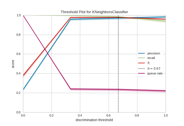
Quick Method
The same functionality above can be achieved with the associated quick method discrimination_threshold. This method will build the DiscriminationThreshold object with the associated arguments, fit it, then (optionally) immediately show it
from yellowbrick.classifier.threshold import discrimination_threshold
from yellowbrick.datasets import load_occupancy
from sklearn.neighbors import KNeighborsClassifier

#Load the classification dataset
X, y = load_occupancy()

# Instantiate the visualizer with the classification model
model = KNeighborsClassifier(3)

discrimination_threshold(model, X, y)
(Source code, png, pdf)
API Reference
DiscriminationThreshold visualizer for probabilistic classifiers.
- class yellowbrick.classifier.threshold.DiscriminationThreshold(estimator, ax=None, n_trials=50, cv=0.1, fbeta=1.0, argmax='fscore', exclude=None, quantiles=array([0.1, 0.5, 0.9]), random_state=None, is_fitted='auto', force_model=False, **kwargs)[source]
Bases:
ModelVisualizerVisualizes how precision, recall, f1 score, and queue rate change as the discrimination threshold increases. For probabilistic, binary classifiers, the discrimination threshold is the probability at which you choose the positive class over the negative. Generally this is set to 50%, but adjusting the discrimination threshold will adjust sensitivity to false positives which is described by the inverse relationship of precision and recall with respect to the threshold.
The visualizer also accounts for variability in the model by running multiple trials with different train and test splits of the data. The variability is visualized using a band such that the curve is drawn as the median score of each trial and the band is from the 10th to 90th percentile.
The visualizer is intended to help users determine an appropriate threshold for decision making (e.g. at what threshold do we have a human review the data), given a tolerance for precision and recall or limiting the number of records to check (the queue rate).
- Parameters
- estimatorestimator
A scikit-learn estimator that should be a classifier. If the model is not a classifier, an exception is raised. If the internal model is not fitted, it is fit when the visualizer is fitted, unless otherwise specified by
is_fitted.- axmatplotlib Axes, default: None
The axes to plot the figure on. If not specified the current axes will be used (or generated if required).
- n_trialsinteger, default: 50
Number of times to shuffle and split the dataset to account for noise in the threshold metrics curves. Note if cv provides > 1 splits, the number of trials will be n_trials * cv.get_n_splits()
- cvfloat or cross-validation generator, default: 0.1
Determines the splitting strategy for each trial. Possible inputs are:
float, to specify the percent of the test split
object to be used as cross-validation generator
This attribute is meant to give flexibility with stratified splitting but if a splitter is provided, it should only return one split and have shuffle set to True.
- fbetafloat, 1.0 by default
The strength of recall versus precision in the F-score.
- argmaxstr or None, default: ‘fscore’
Annotate the threshold maximized by the supplied metric (see exclude for the possible metrics to use). If None or passed to exclude, will not annotate the graph.
- excludestr or list, optional
Specify metrics to omit from the graph, can include:
"precision""recall""queue_rate""fscore"
Excluded metrics will not be displayed in the graph, nor will they be available in
thresholds_; however, they will be computed on fit.- quantilessequence, default: np.array([0.1, 0.5, 0.9])
Specify the quantiles to view model variability across a number of trials. Must be monotonic and have three elements such that the first element is the lower bound, the second is the drawn curve, and the third is the upper bound. By default the curve is drawn at the median, and the bounds from the 10th percentile to the 90th percentile.
- random_stateint, optional
Used to seed the random state for shuffling the data while composing different train and test splits. If supplied, the random state is incremented in a deterministic fashion for each split.
Note that if a splitter is provided, it’s random state will also be updated with this random state, even if it was previously set.
- is_fittedbool or str, default=”auto”
Specify if the wrapped estimator is already fitted. If False, the estimator will be fit when the visualizer is fit, otherwise, the estimator will not be modified. If “auto” (default), a helper method will check if the estimator is fitted before fitting it again.
- force_modelbool, default: False
Do not check to ensure that the underlying estimator is a classifier. This will prevent an exception when the visualizer is initialized but may result in unexpected or unintended behavior.
- kwargsdict
Keyword arguments passed to the visualizer base classes.
Notes
The term “discrimination threshold” is rare in the literature. Here, we use it to mean the probability at which the positive class is selected over the negative class in binary classification.
Classification models must implement either a
decision_functionorpredict_probamethod in order to be used with this class. AYellowbrickTypeErroris raised otherwise.Caution
This method only works for binary, probabilistic classifiers.
See also
For a thorough explanation of discrimination thresholds, see: Visualizing Machine Learning Thresholds to Make Better Business Decisions by Insight Data.
- Attributes
- thresholds_array
The uniform thresholds identified by each of the trial runs.
- cv_scores_dict of arrays of
len(thresholds_) The values for all included metrics including the upper and lower bounds of the metrics defined by quantiles.
- finalize(**kwargs)[source]
Sets a title and axis labels on the visualizer and ensures that the axis limits are scaled to valid threshold values.
- Parameters
- kwargs: generic keyword arguments.
Notes
Generally this method is called from show and not directly by the user.
- fit(X, y, **kwargs)[source]
Fit is the entry point for the visualizer. Given instances described by X and binary classes described in the target y, fit performs n trials by shuffling and splitting the dataset then computing the precision, recall, f1, and queue rate scores for each trial. The scores are aggregated by the quantiles expressed then drawn.
- Parameters
- Xndarray or DataFrame of shape n x m
A matrix of n instances with m features
- yndarray or Series of length n
An array or series of target or class values. The target y must be a binary classification target.
- kwargs: dict
keyword arguments passed to Scikit-Learn API.
- Returns
- selfinstance
Returns the instance of the visualizer
- raises: YellowbrickValueError
If the target y is not a binary classification target.
- yellowbrick.classifier.threshold.discrimination_threshold(estimator, X, y, ax=None, n_trials=50, cv=0.1, fbeta=1.0, argmax='fscore', exclude=None, quantiles=array([0.1, 0.5, 0.9]), random_state=None, is_fitted='auto', force_model=False, show=True, **kwargs)[source]
Discrimination Threshold
Visualizes how precision, recall, f1 score, and queue rate change as the discrimination threshold increases. For probabilistic, binary classifiers, the discrimination threshold is the probability at which you choose the positive class over the negative. Generally this is set to 50%, but adjusting the discrimination threshold will adjust sensitivity to false positives which is described by the inverse relationship of precision and recall with respect to the threshold.
See also
See DiscriminationThreshold for more details.
- Parameters
- estimatorestimator
A scikit-learn estimator that should be a classifier. If the model is not a classifier, an exception is raised. If the internal model is not fitted, it is fit when the visualizer is fitted, unless otherwise specified by
is_fitted.- Xndarray or DataFrame of shape n x m
A matrix of n instances with m features
- yndarray or Series of length n
An array or series of target or class values. The target y must be a binary classification target.
- axmatplotlib Axes, default: None
The axes to plot the figure on. If not specified the current axes will be used (or generated if required).
- n_trialsinteger, default: 50
Number of times to shuffle and split the dataset to account for noise in the threshold metrics curves. Note if cv provides > 1 splits, the number of trials will be n_trials * cv.get_n_splits()
- cvfloat or cross-validation generator, default: 0.1
Determines the splitting strategy for each trial. Possible inputs are:
float, to specify the percent of the test split
object to be used as cross-validation generator
This attribute is meant to give flexibility with stratified splitting but if a splitter is provided, it should only return one split and have shuffle set to True.
- fbetafloat, 1.0 by default
The strength of recall versus precision in the F-score.
- argmaxstr or None, default: ‘fscore’
Annotate the threshold maximized by the supplied metric (see exclude for the possible metrics to use). If None or passed to exclude, will not annotate the graph.
- excludestr or list, optional
Specify metrics to omit from the graph, can include:
"precision""recall""queue_rate""fscore"
Excluded metrics will not be displayed in the graph, nor will they be available in
thresholds_; however, they will be computed on fit.- quantilessequence, default: np.array([0.1, 0.5, 0.9])
Specify the quantiles to view model variability across a number of trials. Must be monotonic and have three elements such that the first element is the lower bound, the second is the drawn curve, and the third is the upper bound. By default the curve is drawn at the median, and the bounds from the 10th percentile to the 90th percentile.
- random_stateint, optional
Used to seed the random state for shuffling the data while composing different train and test splits. If supplied, the random state is incremented in a deterministic fashion for each split.
Note that if a splitter is provided, it’s random state will also be updated with this random state, even if it was previously set.
- is_fittedbool or str, default=”auto”
Specify if the wrapped estimator is already fitted. If False, the estimator will be fit when the visualizer is fit, otherwise, the estimator will not be modified. If “auto” (default), a helper method will check if the estimator is fitted before fitting it again.
- force_modelbool, default: False
Do not check to ensure that the underlying estimator is a classifier. This will prevent an exception when the visualizer is initialized but may result in unexpected or unintended behavior.
- showbool, default: True
If True, calls
show(), which in turn callsplt.show()however you cannot callplt.savefigfrom this signature, norclear_figure. If False, simply callsfinalize()- kwargsdict
Keyword arguments passed to the visualizer base classes.
- Returns
- vizDiscriminationThreshold
Returns the fitted and finalized visualizer object.
Notes
The term “discrimination threshold” is rare in the literature. Here, we use it to mean the probability at which the positive class is selected over the negative class in binary classification.
Classification models must implement either a
decision_functionorpredict_probamethod in order to be used with this class. AYellowbrickTypeErroris raised otherwise.See also
For a thorough explanation of discrimination thresholds, see: Visualizing Machine Learning Thresholds to Make Better Business Decisions by Insight Data.
Examples
>>> from yellowbrick.classifier.threshold import discrimination_threshold
>>> from sklearn.linear_model import LogisticRegression
>>> from yellowbrick.datasets import load_occupancy
>>> X, y = load_occupancy()
>>> model = LogisticRegression(multi_class="auto", solver="liblinear")
>>> discrimination_threshold(model, X, y)