Manifold Visualization
The Manifold visualizer provides high dimensional visualization using
manifold learning
to embed instances described by many dimensions into 2, thus allowing the
creation of a scatter plot that shows latent structures in data. Unlike
decomposition methods such as PCA and SVD, manifolds generally use
nearest-neighbors approaches to embedding, allowing them to capture non-linear
structures that would be otherwise lost. The projections that are produced
can then be analyzed for noise or separability to determine if it is possible
to create a decision space in the data.
Visualizer |
|
Quick Method |
|
Models |
Classification, Regression |
Workflow |
Feature Engineering |
The Manifold visualizer allows access to all currently available
scikit-learn manifold implementations by specifying the manifold as a string to the visualizer. The currently implemented default manifolds are as follows:
Manifold |
Description |
|
Locally Linear Embedding (LLE) uses many local linear decompositions to preserve globally non-linear structures. |
|
LTSA LLE: local tangent space alignment is similar to LLE in that it uses locality to preserve neighborhood distances. |
|
Hessian LLE an LLE regularization method that applies a hessian-based quadratic form at each neighborhood |
|
Modified LLE applies a regularization parameter to LLE. |
|
Isomap seeks a lower dimensional embedding that maintains geometric distances between each instance. |
|
MDS: multi-dimensional scaling uses similarity to plot points that are near to each other close in the embedding. |
|
Spectral Embedding a discrete approximation of the low dimensional manifold using a graph representation. |
|
t-SNE: converts the similarity of points into probabilities then uses those probabilities to create an embedding. |
Each manifold algorithm produces a different embedding and takes advantage of different properties of the underlying data. Generally speaking, it requires multiple attempts on new data to determine the manifold that works best for the structures latent in your data. Note however, that different manifold algorithms have different time, complexity, and resource requirements.
Manifolds can be used on many types of problems, and the color used in the scatter plot can describe the target instance. In an unsupervised or clustering problem, a single color is used to show structure and overlap. In a classification problem discrete colors are used for each class. In a regression problem, a color map can be used to describe points as a heat map of their regression values.
Discrete Target
In a classification or clustering problem, the instances can be described by discrete labels - the classes or categories in the supervised problem, or the clusters they belong to in the unsupervised version. The manifold visualizes this by assigning a color to each label and showing the labels in a legend.
from yellowbrick.features import Manifold
from yellowbrick.datasets import load_occupancy

# Load the classification dataset
X, y = load_occupancy()
classes = ["unoccupied", "occupied"]

# Instantiate the visualizer
viz = Manifold(manifold="tsne", classes=classes)

viz.fit_transform(X, y)  # Fit the data to the visualizer
viz.show()               # Finalize and render the figure
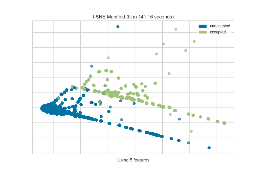
The visualization also displays the amount of time it takes to generate the
embedding; as you can see, this can take a long time even for relatively
small datasets. One tip is scale your data using the StandardScalar;
another is to sample your instances (e.g. using train_test_split to
preserve class stratification) or to filter features to decrease sparsity in
the dataset.
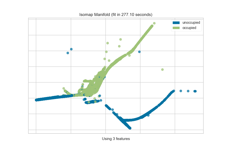
One common mechanism is to use SelectKBest to select the features that have
a statistical correlation with the target dataset. For example, we can use
the f_classif score to find the 3 best features in our occupancy dataset.
from sklearn.pipeline import Pipeline
from sklearn.feature_selection import f_classif, SelectKBest

from yellowbrick.features import Manifold
from yellowbrick.datasets import load_occupancy

# Load the classification dataset
X, y = load_occupancy()
classes = ["unoccupied", "occupied"]

# Create a pipeline
model = Pipeline([
    ("selectk", SelectKBest(k=3, score_func=f_classif)),
    ("viz", Manifold(manifold="isomap", n_neighbors=10, classes=classes)),
])

model.fit_transform(X, y)          # Fit the data to the model
model.named_steps['viz'].show()   # Finalize and render the figure
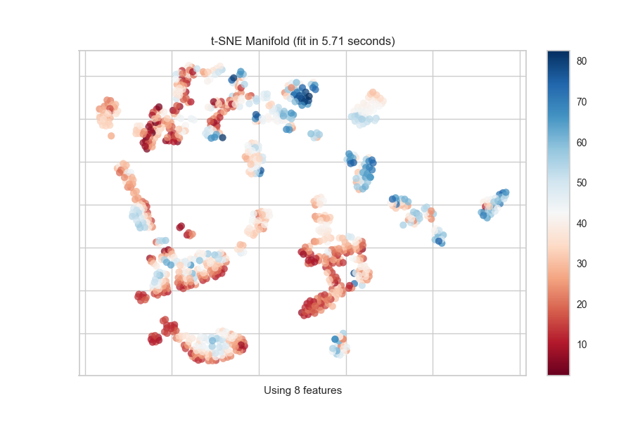
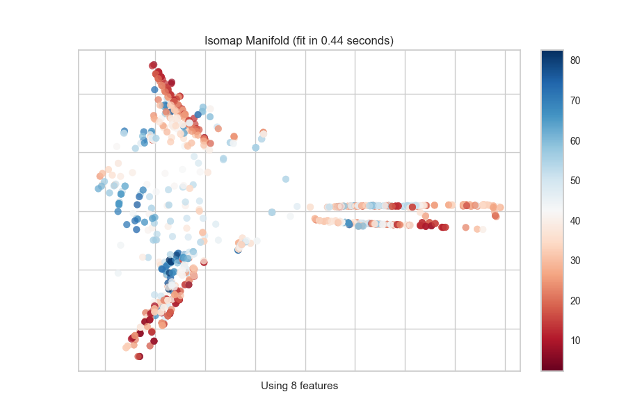
Continuous Target
For a regression target or to specify color as a heat-map of continuous
values, specify target_type="continuous". Note that by default the param
target_type="auto" is set, which determines if the target is discrete or
continuous by counting the number of unique values in y.
from yellowbrick.features import Manifold
from yellowbrick.datasets import load_concrete

# Load the regression dataset
X, y = load_concrete()

# Instantiate the visualizer
viz = Manifold(manifold="isomap", n_neighbors=10)

viz.fit_transform(X, y)  # Fit the data to the visualizer
viz.show()               # Finalize and render the figure

Quick Method
The same functionality above can be achieved with the associated quick method manifold_embedding. This method will build the Manifold object with the associated arguments, fit it, then (optionally) immediately show the visualization.
from yellowbrick.features.manifold import manifold_embedding
from yellowbrick.datasets import load_concrete

# Load the regression dataset
X, y = load_concrete()

# Instantiate the visualizer
manifold_embedding(X, y, manifold="isomap", n_neighbors=10)
API Reference
Use manifold algorithms for high dimensional visualization.
- class yellowbrick.features.manifold.Manifold(ax=None, manifold='mds', n_neighbors=None, features=None, classes=None, colors=None, colormap=None, target_type='auto', projection=2, alpha=0.75, random_state=None, colorbar=True, **kwargs)[source]
Bases:
ProjectionVisualizerThe Manifold visualizer provides high dimensional visualization for feature analysis by embedding data into 2 dimensions using the sklearn.manifold package for manifold learning. In brief, manifold learning algorithms are unsuperivsed approaches to non-linear dimensionality reduction (unlike PCA or SVD) that help visualize latent structures in data.
The manifold algorithm used to do the embedding in scatter plot space can either be a transformer or a string representing one of the already specified manifolds as follows:
Manifold
Description
"lle""ltsa""hessian""modified""isomap""mds""spectral""tsne"Each of these algorithms embeds non-linear relationships in different ways, allowing for an exploration of various structures in the feature space. Note however, that each of these algorithms has different time, memory and complexity requirements; take special care when using large datasets!
The Manifold visualizer also shows the specified target (if given) as the color of the scatter plot. If a classification or clustering target is given, then discrete colors will be used with a legend. If a regression or continuous target is specified, then a colormap and colorbar will be shown.
- Parameters
- axmatplotlib Axes, default: None
The axes to plot the figure on. If None, the current axes will be used or generated if required.
- manifoldstr or Transformer, default: “mds”
Specify the manifold algorithm to perform the embedding. Either one of the strings listed in the table above, or an actual scikit-learn transformer. The constructed manifold is accessible with the manifold property, so as to modify hyperparameters before fit.
- n_neighborsint, default: None
Many manifold algorithms are nearest neighbors based, for those that are, this parameter specfies the number of neighbors to use in the embedding. If n_neighbors is not specified for those embeddings, it is set to 5 and a warning is issued. If the manifold algorithm doesn’t use nearest neighbors, then this parameter is ignored.
- featureslist, default: None
The names of the features specified by the columns of the input dataset. This length of this list must match the number of columns in X, otherwise an exception will be raised on
fit().- classeslist, default: None
The class labels for each class in y, ordered by sorted class index. These names act as a label encoder for the legend, identifying integer classes or renaming string labels. If omitted, the class labels will be taken from the unique values in y.
Note that the length of this list must match the number of unique values in y, otherwise an exception is raised. This parameter is only used in the discrete target type case and is ignored otherwise.
- colorslist or tuple, default: None
A single color to plot all instances as or a list of colors to color each instance according to its class in the discrete case or as an ordered colormap in the sequential case. If not enough colors per class are specified then the colors are treated as a cycle.
- colormapstring or cmap, default: None
The colormap used to create the individual colors. In the discrete case it is used to compute the number of colors needed for each class and in the continuous case it is used to create a sequential color map based on the range of the target.
- target_typestr, default: “auto”
Specify the type of target as either “discrete” (classes) or “continuous” (real numbers, usually for regression). If “auto”, then it will attempt to determine the type by counting the number of unique values.
If the target is discrete, the colors are returned as a dict with classes being the keys. If continuous the colors will be list having value of color for each point. In either case, if no target is specified, then color will be specified as the first color in the color cycle.
- projectionint or string, default: 2
The number of axes to project into, either 2d or 3d. To plot 3d plots with matplotlib, please ensure a 3d axes is passed to the visualizer, otherwise one will be created using the current figure.
- alphafloat, default: 0.75
Specify a transparency where 1 is completely opaque and 0 is completely transparent. This property makes densely clustered points more visible.
- random_stateint or RandomState, default: None
Fixes the random state for stochastic manifold algorithms.
- colorbarbool, default: True
If the target_type is “continous” draw a colorbar to the right of the scatter plot. The colobar axes is accessible using the cax property.
- kwargsdict
Keyword arguments passed to the base class and may influence the feature visualization properties.
Notes
Specifying the target as
'continuous'or'discrete'will influence how the visualizer is finally displayed, don’t rely on the automatic determination from the Manifold!Scaling your data with the standard scalar before applying it to the visualizer is a great way of increasing performance. Additionally using the
SelectKBesttransformer may also improve performance and lead to better visualizations.Warning
Manifold visualizers have extremly varying time, resource, and complexity requirements. Sampling data or features may be necessary in order to finish a manifold computation.
See also
The Scikit-Learn discussion on Manifold Learning.
Examples
>>> viz = Manifold(manifold='isomap', target='discrete')
>>> viz.fit_transform(X, y)
>>> viz.show()
- Attributes
- fit_time_yellowbrick.utils.timer.Timer
The amount of time in seconds it took to fit the Manifold.
- classes_ndarray, shape (n_classes,)
The class labels that define the discrete values in the target. Only available if the target type is discrete. This is guaranteed to be strings even if the classes are a different type.
- features_ndarray, shape (n_features,)
The names of the features discovered or used in the visualizer that can be used as an index to access or modify data in X. If a user passes feature names in, those features are used. Otherwise the columns of a DataFrame are used or just simply the indices of the data array.
- range_(min y, max y)
A tuple that describes the minimum and maximum values in the target. Only available if the target type is continuous.
- ALGORITHMS = {'hessian': LocallyLinearEmbedding(method='hessian'), 'isomap': Isomap(), 'lle': LocallyLinearEmbedding(), 'ltsa': LocallyLinearEmbedding(method='ltsa'), 'mds': MDS(), 'modified': LocallyLinearEmbedding(method='modified'), 'spectral': SpectralEmbedding(), 'tsne': TSNE(init='pca')}
- draw(Xp, y=None)[source]
Draws the points described by Xp and colored by the points in y. Can be called multiple times before finalize to add more scatter plots to the axes, however
fit()must be called before use.- Parameters
- Xparray-like of shape (n, 2) or (n, 3)
The matrix produced by the
transform()method.- yarray-like of shape (n,), optional
The target, used to specify the colors of the points.
- Returns
- self.axmatplotlib Axes object
Returns the axes that the scatter plot was drawn on.
- fit(X, y=None, **kwargs)[source]
Fits the manifold on X and transforms the data to plot it on the axes. See fit_transform() for more details.
- Parameters
- Xarray-like of shape (n, m)
A matrix or data frame with n instances and m features
- yarray-like of shape (n,), optional
A vector or series with target values for each instance in X. This vector is used to determine the color of the points in X.
- Returns
- selfManifold
Returns the visualizer object.
- fit_transform(X, y=None, **kwargs)[source]
Fits the manifold on X and transforms the data to plot it on the axes. The optional y specified can be used to declare discrete colors. If the target is set to ‘auto’, this method also determines the target type, and therefore what colors will be used.
Note also that fit records the amount of time it takes to fit the manifold and reports that information in the visualization.
- Parameters
- Xarray-like of shape (n, m)
A matrix or data frame with n instances and m features
- yarray-like of shape (n,), optional
A vector or series with target values for each instance in X. This vector is used to determine the color of the points in X.
- Returns
- Xprimearray-like of shape (n, 2)
Returns the 2-dimensional embedding of the instances.
- property manifold
Property containing the manifold transformer constructed from the supplied hyperparameter. Use this property to modify the manifold before fit with
manifold.set_params().
- transform(X, y=None, **kwargs)[source]
Returns the transformed data points from the manifold embedding.
- Parameters
- Xarray-like of shape (n, m)
A matrix or data frame with n instances and m features
- yarray-like of shape (n,), optional
The target, used to specify the colors of the points.
- Returns
- Xprimearray-like of shape (n, 2)
Returns the 2-dimensional embedding of the instances.
- yellowbrick.features.manifold.manifold_embedding(X, y=None, ax=None, manifold='mds', n_neighbors=None, features=None, classes=None, colors=None, colormap=None, target_type='auto', projection=2, alpha=0.75, random_state=None, colorbar=True, show=True, **kwargs)[source]
Quick method for Manifold visualizer.
The Manifold visualizer provides high dimensional visualization for feature analysis by embedding data into 2 dimensions using the sklearn.manifold package for manifold learning. In brief, manifold learning algorithms are unsuperivsed approaches to non-linear dimensionality reduction (unlike PCA or SVD) that help visualize latent structures in data.
See also
See Manifold for more details.
- Parameters
- Xarray-like of shape (n, m)
A matrix or data frame with n instances and m features where m > 2.
- yarray-like of shape (n,), optional
A vector or series with target values for each instance in X. This vector is used to determine the color of the points in X.
- axmatplotlib.Axes, default: None
The axis to plot the figure on. If None is passed in the current axes will be used (or generated if required).
- manifoldstr or Transformer, default: “lle”
Specify the manifold algorithm to perform the embedding. Either one of the strings listed in the table above, or an actual scikit-learn transformer. The constructed manifold is accessible with the manifold property, so as to modify hyperparameters before fit.
- n_neighborsint, default: None
Many manifold algorithms are nearest neighbors based, for those that are, this parameter specfies the number of neighbors to use in the embedding. If n_neighbors is not specified for those embeddings, it is set to 5 and a warning is issued. If the manifold algorithm doesn’t use nearest neighbors, then this parameter is ignored.
- featureslist, default: None
The names of the features specified by the columns of the input dataset. This length of this list must match the number of columns in X, otherwise an exception will be raised on
fit().- classeslist, default: None
The class labels for each class in y, ordered by sorted class index. These names act as a label encoder for the legend, identifying integer classes or renaming string labels. If omitted, the class labels will be taken from the unique values in y.
Note that the length of this list must match the number of unique values in y, otherwise an exception is raised. This parameter is only used in the discrete target type case and is ignored otherwise.
- colorslist or tuple, default: None
A single color to plot all instances as or a list of colors to color each instance according to its class in the discrete case or as an ordered colormap in the sequential case. If not enough colors per class are specified then the colors are treated as a cycle.
- colormapstring or cmap, default: None
The colormap used to create the individual colors. In the discrete case it is used to compute the number of colors needed for each class and in the continuous case it is used to create a sequential color map based on the range of the target.
- target_typestr, default: “auto”
Specify the type of target as either “discrete” (classes) or “continuous” (real numbers, usually for regression). If “auto”, then it will attempt to determine the type by counting the number of unique values.
If the target is discrete, the colors are returned as a dict with classes being the keys. If continuous the colors will be list having value of color for each point. In either case, if no target is specified, then color will be specified as the first color in the color cycle.
- projectionint or string, default: 2
The number of axes to project into, either 2d or 3d. To plot 3d plots with matplotlib, please ensure a 3d axes is passed to the visualizer, otherwise one will be created using the current figure.
- alphafloat, default: 0.75
Specify a transparency where 1 is completely opaque and 0 is completely transparent. This property makes densely clustered points more visible.
- random_stateint or RandomState, default: None
Fixes the random state for stochastic manifold algorithms.
- colorbarbool, default: True
If the target_type is “continous” draw a colorbar to the right of the scatter plot. The colobar axes is accessible using the cax property.
- show: bool, default: True
If True, calls
show(), which in turn callsplt.show()however you cannot callplt.savefigfrom this signature, norclear_figure. If False, simply callsfinalize()- kwargsdict
Keyword arguments passed to the base class and may influence the feature visualization properties.
- Returns
- vizManifold
Returns the fitted, finalized visualizer