Parallel Coordinates
Parallel coordinates is multi-dimensional feature visualization technique where the vertical axis is duplicated horizontally for each feature. Instances are displayed as a single line segment drawn from each vertical axes to the location representing their value for that feature. This allows many dimensions to be visualized at once; in fact given infinite horizontal space (e.g. a scrolling window), technically an infinite number of dimensions can be displayed!
Data scientists use this method to detect clusters of instances that have similar classes, and to note features that have high variance or different distributions. We can see this in action after first loading our occupancy classification dataset.
Visualizer |
|
Quick Method |
|
Models |
Classification |
Workflow |
Feature analysis |
from yellowbrick.features import ParallelCoordinates
from yellowbrick.datasets import load_occupancy

# Load the classification data set
X, y = load_occupancy()

# Specify the features of interest and the classes of the target
features = [
    "temperature", "relative humidity", "light", "CO2", "humidity"
]
classes = ["unoccupied", "occupied"]

# Instantiate the visualizer
visualizer = ParallelCoordinates(
    classes=classes, features=features, sample=0.05, shuffle=True
)

# Fit and transform the data to the visualizer
visualizer.fit_transform(X, y)

# Finalize the title and axes then display the visualization
visualizer.show()
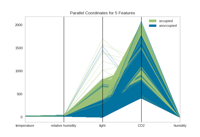
(Source code, png, pdf)
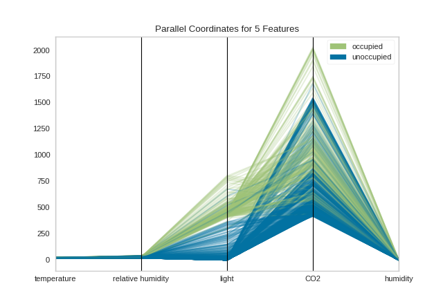
By inspecting the visualization closely, we can see that the combination of transparency and overlap gives us the sense of groups of similar instances, sometimes referred to as “braids”. If there are distinct braids of different classes, it suggests that there is enough separability that a classification algorithm might be able to discern between each class.
Unfortunately, as we inspect this class, we can see that the domain of each feature may make the visualization hard to interpret. In the above visualization, the domain of the light feature is from in [0, 1600], far larger than the range of temperature in [50, 96]. To solve this problem, each feature should be scaled or normalized so they are approximately in the same domain.
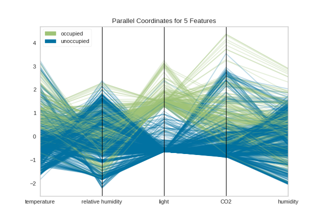
Normalization techniques can be directly applied to the visualizer without pre-transforming the data (though you could also do this) by using the normalize parameter. Several transformers are available; try using minmax, maxabs, standard, l1, or l2 normalization to change perspectives in the parallel coordinates as follows:
from yellowbrick.features import ParallelCoordinates
from yellowbrick.datasets import load_occupancy

# Load the classification data set
X, y = load_occupancy()

# Specify the features of interest and the classes of the target
features = [
    "temperature", "relative humidity", "light", "CO2", "humidity"
]
classes = ["unoccupied", "occupied"]

# Instantiate the visualizer
visualizer = ParallelCoordinates(
    classes=classes, features=features,
    normalize='standard', sample=0.05, shuffle=True,
)

# Fit the visualizer and display it
visualizer.fit_transform(X, y)
visualizer.show()
(Source code, png, pdf)

Now we can see that each feature is in the range [-3, 3] where the mean of the feature is set to zero and each feature has a unit variance applied between [-1, 1] (because we’re using the StandardScaler via the standard normalize parameter). This version of parallel coordinates gives us a much better sense of the distribution of the features and if any features are highly variable with respect to any one class.
Faster Parallel Coordinates
Parallel coordinates can take a long time to draw since each instance is represented by a line for each feature. Worse, this time is not well spent since a lot of overlap in the visualization makes the parallel coordinates less understandable. We propose two solutions to this:
Use
sample=0.2andshuffle=Trueparameters to shuffle and sample the dataset being drawn on the figure. The sample parameter will perform a uniform random sample of the data, selecting the percent specified.Use the
fast=Trueparameter to enable “fast drawing mode”.
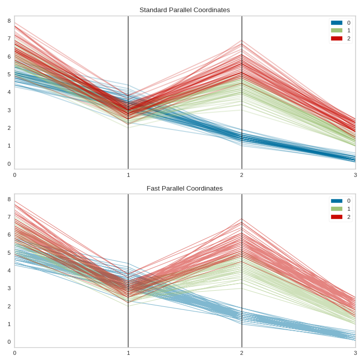
The “fast” drawing mode vastly improves the performance of the parallel coordinates drawing algorithm by drawing each line segment by class rather than each instance individually. However, this improved performance comes at a cost, as the visualization produced is subtly different; compare the visualizations in fast and standard drawing modes below:
(Source code, png, pdf)

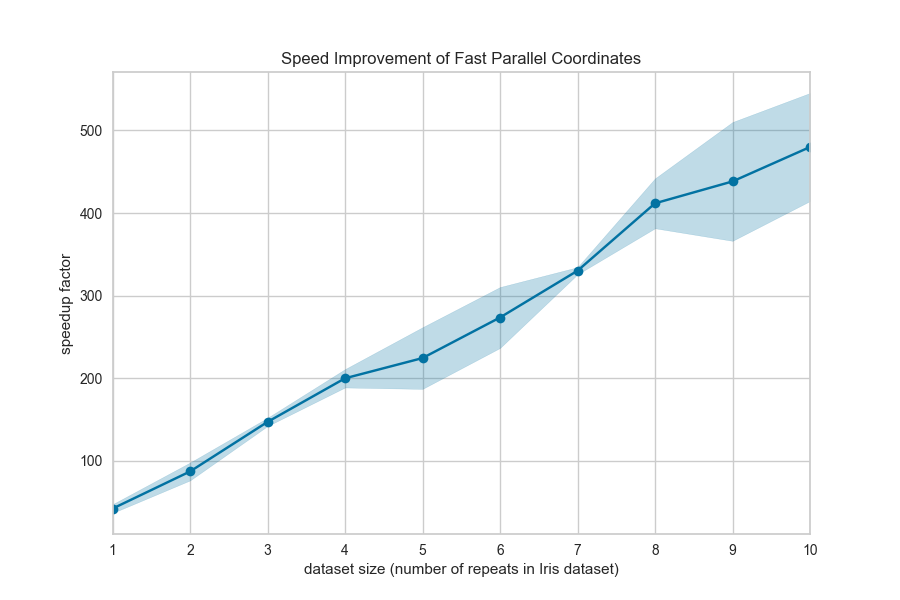
As you can see the “fast” drawing algorithm does not have the same build up of color density where instances of the same class intersect. Because there is only one line per class, there is only a darkening effect between classes. This can lead to a different interpretation of the plot, though it still may be effective for analytical purposes, particularly when you’re plotting a lot of data. Needless to say, the performance benefits are dramatic:
Quick Method
The same functionality above can be achieved with the associated quick method parallel_coordinates. This method
will build the ParallelCoordinates object with the associated arguments, fit it, then (optionally) immediately
show it.
from yellowbrick.features.pcoords import parallel_coordinates
from yellowbrick.datasets import load_occupancy

# Load the classification data set
X, y = load_occupancy()

# Specify the features of interest and the classes of the target
features = [
    "temperature", "relative humidity", "light", "CO2", "humidity"
]
classes = ["unoccupied", "occupied"]

# Instantiate the visualizer
visualizer = parallel_coordinates(X, y, classes=classes, features=features)
(Source code, png, pdf)

API Reference
Implementation of parallel coordinates for multi-dimensional feature analysis.
- class yellowbrick.features.pcoords.ParallelCoordinates(ax=None, features=None, classes=None, normalize=None, sample=1.0, random_state=None, shuffle=False, colors=None, colormap=None, alpha=None, fast=False, vlines=True, vlines_kwds=None, **kwargs)[source]
Bases:
DataVisualizerParallel coordinates displays each feature as a vertical axis spaced evenly along the horizontal, and each instance as a line drawn between each individual axis. This allows you to detect braids of similar instances and separability that suggests a good classification problem.
- Parameters
- axmatplotlib Axes, default: None
The axis to plot the figure on. If None is passed in the current axes will be used (or generated if required).
- featureslist, default: None
a list of feature names to use If a DataFrame is passed to fit and features is None, feature names are selected as the columns of the DataFrame.
- classeslist, default: None
a list of class names for the legend The class labels for each class in y, ordered by sorted class index. These names act as a label encoder for the legend, identifying integer classes or renaming string labels. If omitted, the class labels will be taken from the unique values in y.
Note that the length of this list must match the number of unique values in y, otherwise an exception is raised.
- normalizestring or None, default: None
specifies which normalization method to use, if any Current supported options are ‘minmax’, ‘maxabs’, ‘standard’, ‘l1’, and ‘l2’.
- samplefloat or int, default: 1.0
specifies how many examples to display from the data If int, specifies the maximum number of samples to display. If float, specifies a fraction between 0 and 1 to display.
- random_stateint, RandomState instance or None
If int, random_state is the seed used by the random number generator; If RandomState instance, random_state is the random number generator; If None, the random number generator is the RandomState instance used by np.random; only used if shuffle is True and sample < 1.0
- shuffleboolean, default: True
specifies whether sample is drawn randomly
- colorslist or tuple, default: None
A single color to plot all instances as or a list of colors to color each instance according to its class. If not enough colors per class are specified then the colors are treated as a cycle.
- colormapstring or cmap, default: None
The colormap used to create the individual colors. If classes are specified the colormap is used to evenly space colors across each class.
- alphafloat, default: None
Specify a transparency where 1 is completely opaque and 0 is completely transparent. This property makes densely clustered lines more visible. If None, the alpha is set to 0.5 in “fast” mode and 0.25 otherwise.
- fastbool, default: False
Fast mode improves the performance of the drawing time of parallel coordinates but produces an image that does not show the overlap of instances in the same class. Fast mode should be used when drawing all instances is too burdensome and sampling is not an option.
- vlinesboolean, default: True
flag to determine vertical line display
- vlines_kwdsdict, default: None
options to style or display the vertical lines, default: None
- kwargsdict
Keyword arguments that are passed to the base class and may influence the visualization as defined in other Visualizers.
Examples
>>> visualizer = ParallelCoordinates()
>>> visualizer.fit(X, y)
>>> visualizer.transform(X)
>>> visualizer.show()
- Attributes
- n_samples_int
number of samples included in the visualization object
- features_ndarray, shape (n_features,)
The names of the features discovered or used in the visualizer that can be used as an index to access or modify data in X. If a user passes feature names in, those features are used. Otherwise the columns of a DataFrame are used or just simply the indices of the data array.
- classes_ndarray, shape (n_classes,)
The class labels that define the discrete values in the target. Only available if the target type is discrete. This is guaranteed to be strings even if the classes are a different type.
- NORMALIZERS = {'l1': Normalizer(norm='l1'), 'l2': Normalizer(), 'maxabs': MaxAbsScaler(), 'minmax': MinMaxScaler(), 'standard': StandardScaler()}
- draw(X, y, **kwargs)[source]
Called from the fit method, this method creates the parallel coordinates canvas and draws each instance and vertical lines on it.
- Parameters
- Xndarray of shape n x m
A matrix of n instances with m features
- yndarray of length n
An array or series of target or class values
- kwargsdict
Pass generic arguments to the drawing method
- draw_classes(X, y, **kwargs)[source]
Draw the instances colored by the target y such that each line is a single class. This is the “fast” mode of drawing, since the number of lines drawn equals the number of classes, rather than the number of instances. However, this drawing method sacrifices inter-class density of points using the alpha parameter.
- Parameters
- Xndarray of shape n x m
A matrix of n instances with m features
- yndarray of length n
An array or series of target or class values
- draw_instances(X, y, **kwargs)[source]
Draw the instances colored by the target y such that each line is a single instance. This is the “slow” mode of drawing, since each instance has to be drawn individually. However, in so doing, the density of instances in braids is more apparent since lines have an independent alpha that is compounded in the figure.
This is the default method of drawing.
- Parameters
- Xndarray of shape n x m
A matrix of n instances with m features
- yndarray of length n
An array or series of target or class values
Notes
This method can be used to draw additional instances onto the parallel coordinates before the figure is finalized.
- finalize(**kwargs)[source]
Performs the final rendering for the multi-axis visualization, including setting and rendering the vertical axes each instance is plotted on. Adds a title, a legend, and manages the grid.
- Parameters
- kwargs: generic keyword arguments.
Notes
Generally this method is called from show and not directly by the user.
- fit(X, y=None, **kwargs)[source]
The fit method is the primary drawing input for the visualization since it has both the X and y data required for the viz and the transform method does not.
- Parameters
- Xndarray or DataFrame of shape n x m
A matrix of n instances with m features
- yndarray or Series of length n
An array or series of target or class values
- kwargsdict
Pass generic arguments to the drawing method
- Returns
- selfinstance
Returns the instance of the transformer/visualizer
- yellowbrick.features.pcoords.parallel_coordinates(X, y, ax=None, features=None, classes=None, normalize=None, sample=1.0, random_state=None, shuffle=False, colors=None, colormap=None, alpha=None, fast=False, vlines=True, vlines_kwds=None, show=True, **kwargs)[source]
Displays each feature as a vertical axis and each instance as a line.
This helper function is a quick wrapper to utilize the ParallelCoordinates Visualizer (Transformer) for one-off analysis.
- Parameters
- Xndarray or DataFrame of shape n x m
A matrix of n instances with m features
- yndarray or Series of length n
An array or series of target or class values
- axmatplotlib Axes, default: None
The axis to plot the figure on. If None is passed in the current axes will be used (or generated if required).
- featureslist, default: None
a list of feature names to use If a DataFrame is passed to fit and features is None, feature names are selected as the columns of the DataFrame.
- classeslist, default: None
a list of class names for the legend If classes is None and a y value is passed to fit then the classes are selected from the target vector.
- normalizestring or None, default: None
specifies which normalization method to use, if any Current supported options are ‘minmax’, ‘maxabs’, ‘standard’, ‘l1’, and ‘l2’.
- samplefloat or int, default: 1.0
specifies how many examples to display from the data If int, specifies the maximum number of samples to display. If float, specifies a fraction between 0 and 1 to display.
- random_stateint, RandomState instance or None
If int, random_state is the seed used by the random number generator; If RandomState instance, random_state is the random number generator; If None, the random number generator is the RandomState instance used by np.random; only used if shuffle is True and sample < 1.0
- shuffleboolean, default: True
specifies whether sample is drawn randomly
- colorslist or tuple, default: None
optional list or tuple of colors to colorize lines Use either color to colorize the lines on a per class basis or colormap to color them on a continuous scale.
- colormapstring or cmap, default: None
optional string or matplotlib cmap to colorize lines Use either color to colorize the lines on a per class basis or colormap to color them on a continuous scale.
- alphafloat, default: None
Specify a transparency where 1 is completely opaque and 0 is completely transparent. This property makes densely clustered lines more visible. If None, the alpha is set to 0.5 in “fast” mode and 0.25 otherwise.
- fastbool, default: False
Fast mode improves the performance of the drawing time of parallel coordinates but produces an image that does not show the overlap of instances in the same class. Fast mode should be used when drawing all instances is too burdensome and sampling is not an option.
- vlinesboolean, default: True
flag to determine vertical line display
- vlines_kwdsdict, default: None
options to style or display the vertical lines, default: None
- showbool, default: True
If True, calls
show(), which in turn callsplt.show()however you cannot callplt.savefigfrom this signature, norclear_figure. If False, simply callsfinalize()- kwargsdict
Keyword arguments that are passed to the base class and may influence the visualization as defined in other Visualizers.
- Returns
- vizParallelCoordinates
Returns the fitted, finalized visualizer