Token Frequency Distribution
A method for visualizing the frequency of tokens within and across corpora is frequency distribution. A frequency distribution tells us the frequency of each vocabulary item in the text. In general, it could count any kind of observable event. It is a distribution because it tells us how the total number of word tokens in the text are distributed across the vocabulary items.
Visualizer |
|
Quick Method |
|
Models |
Text |
Workflow |
Text Analysis |
Note
The FreqDistVisualizer does not perform any normalization or vectorization, and it expects text that has already been count vectorized.
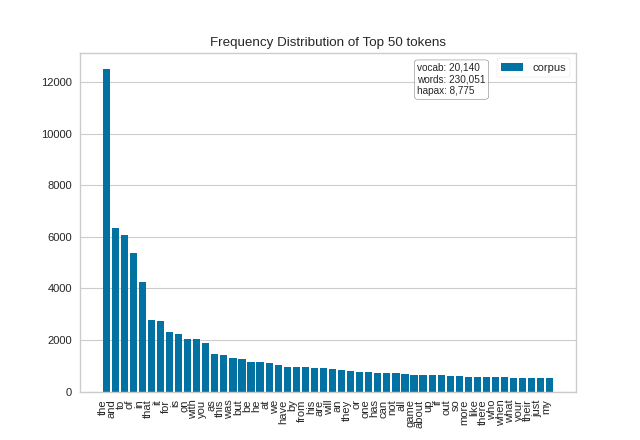
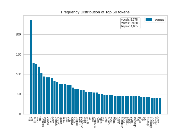
We first instantiate a FreqDistVisualizer object, and then call fit() on that object with the count vectorized documents and the features (i.e. the words from the corpus), which computes the frequency distribution. The visualizer then plots a bar chart of the top 50 most frequent terms in the corpus, with the terms listed along the x-axis and frequency counts depicted at y-axis values. As with other Yellowbrick visualizers, when the user invokes show(), the finalized visualization is shown. Note that in this plot and in the subsequent one, we can orient our plot vertically by passing in orient='v' on instantiation (the plot will orient horizontally by default):
from sklearn.feature_extraction.text import CountVectorizer

from yellowbrick.text import FreqDistVisualizer
from yellowbrick.datasets import load_hobbies

# Load the text data
corpus = load_hobbies()

vectorizer = CountVectorizer()
docs       = vectorizer.fit_transform(corpus.data)
features   = vectorizer.get_feature_names()

visualizer = FreqDistVisualizer(features=features, orient='v')
visualizer.fit(docs)
visualizer.show()
(Source code, png, pdf)

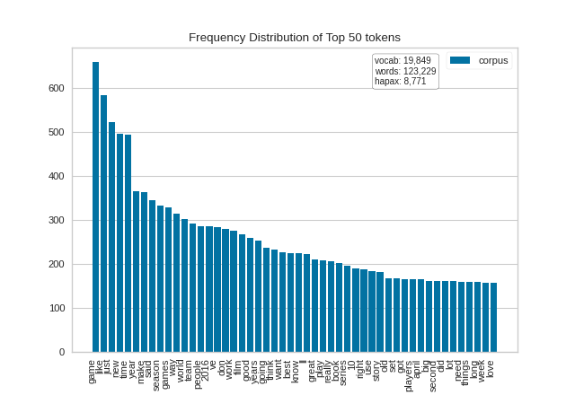
It is interesting to compare the results of the FreqDistVisualizer before and after stopwords have been removed from the corpus:
(Source code, png, pdf)
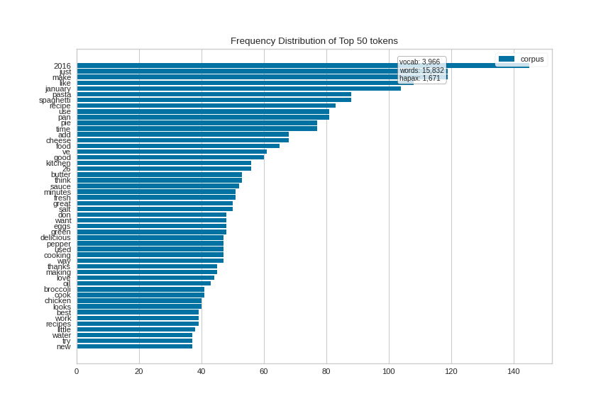
It is also interesting to explore the differences in tokens across a corpus. The hobbies corpus that comes with Yellowbrick has already been categorized (try corpus.target), so let’s visually compare the differences in the frequency distributions for two of the categories: “cooking” and “gaming”.
Here is the plot for the cooking corpus (oriented horizontally this time):
(Source code, png, pdf)

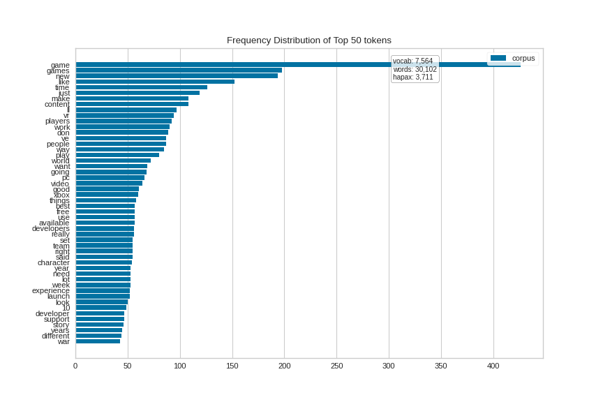
And for the gaming corpus (again oriented horizontally):
(Source code, png, pdf)

Quick Method
Similar functionality as above can be achieved in one line using the associated quick method, freqdist. This method will instantiate with features(words) and fit a FreqDistVisualizer visualizer on the documents).
from collections import defaultdict

from sklearn.feature_extraction.text import CountVectorizer

from yellowbrick.text import freqdist
from yellowbrick.datasets import load_hobbies

# Load the text data
corpus = load_hobbies()

# Create a dict to map target labels to documents of that category
hobbies = defaultdict(list)
for text, label in zip(corpus.data, corpus.target):
    hobbies[label].append(text)

vectorizer = CountVectorizer(stop_words='english')
docs       = vectorizer.fit_transform(text for text in hobbies['cinema'])
features   = vectorizer.get_feature_names()

freqdist(features, docs, orient='v')
(Source code, png, pdf)

API Reference
Implementations of frequency distributions for text visualization
- class yellowbrick.text.freqdist.FrequencyVisualizer(features, ax=None, n=50, orient='h', color=None, **kwargs)[source]
Bases:
TextVisualizerA frequency distribution tells us the frequency of each vocabulary item in the text. In general, it could count any kind of observable event. It is a distribution because it tells us how the total number of word tokens in the text are distributed across the vocabulary items.
- Parameters
- featureslist, default: None
The list of feature names from the vectorizer, ordered by index. E.g. a lexicon that specifies the unique vocabulary of the corpus. This can be typically fetched using the
get_feature_names()method of the transformer in Scikit-Learn.- axmatplotlib axes, default: None
The axes to plot the figure on.
- n: integer, default: 50
Top N tokens to be plotted.
- orient‘h’ or ‘v’, default: ‘h’
Specifies a horizontal or vertical bar chart.
- colorstring
Specify color for bars
- kwargsdict
Pass any additional keyword arguments to the super class.
- These parameters can be influenced later on in the visualization
- process, but can and should be set as early as possible.
- count(X)[source]
Called from the fit method, this method gets all the words from the corpus and their corresponding frequency counts.
- Parameters
- Xndarray or masked ndarray
Pass in the matrix of vectorized documents, can be masked in order to sum the word frequencies for only a subset of documents.
- Returns
- countsarray
A vector containing the counts of all words in X (columns)
- draw(**kwargs)[source]
Called from the fit method, this method creates the canvas and draws the distribution plot on it.
- Parameters
- kwargs: generic keyword arguments.
- finalize(**kwargs)[source]
The finalize method executes any subclass-specific axes finalization steps. The user calls show & show calls finalize.
- Parameters
- kwargs: generic keyword arguments.
- fit(X, y=None)[source]
The fit method is the primary drawing input for the frequency distribution visualization. It requires vectorized lists of documents and a list of features, which are the actual words from the original corpus (needed to label the x-axis ticks).
- Parameters
- Xndarray or DataFrame of shape n x m
A matrix of n instances with m features representing the corpus of frequency vectorized documents.
- yndarray or DataFrame of shape n
Labels for the documents for conditional frequency distribution.
Notes
Note
Text documents must be vectorized before
fit().
- yellowbrick.text.freqdist.freqdist(features, X, y=None, ax=None, n=50, orient='h', color=None, show=True, **kwargs)[source]
Displays frequency distribution plot for text.
This helper function is a quick wrapper to utilize the FreqDist Visualizer (Transformer) for one-off analysis.
- Parameters
- featureslist, default: None
The list of feature names from the vectorizer, ordered by index. E.g. a lexicon that specifies the unique vocabulary of the corpus. This can be typically fetched using the
get_feature_names()method of the transformer in Scikit-Learn.- X: ndarray or DataFrame of shape n x m
A matrix of n instances with m features. In the case of text, X is a list of list of already preprocessed words
- y: ndarray or Series of length n
An array or series of target or class values
- axmatplotlib axes, default: None
The axes to plot the figure on.
- n: integer, default: 50
Top N tokens to be plotted.
- orient‘h’ or ‘v’, default: ‘h’
Specifies a horizontal or vertical bar chart.
- colorstring
Specify color for bars
- show: bool, default: True
If True, calls
show(), which in turn callsplt.show()however you cannot callplt.savefigfrom this signature, norclear_figure. If False, simply callsfinalize()- kwargs: dict
Keyword arguments passed to the super class.
- Returns
- visualizer: FreqDistVisualizer
Returns the fitted, finalized visualizer