t-SNE Corpus Visualization
Visualizer |
|
Quick Method |
|
Models |
Decomposition |
Workflow |
Feature Engineering/Selection |
One very popular method for visualizing document similarity is to use t-distributed stochastic neighbor embedding, t-SNE. Scikit-learn implements this decomposition method as the sklearn.manifold.TSNE transformer. By decomposing high-dimensional document vectors into 2 dimensions using probability distributions from both the original dimensionality and the decomposed dimensionality, t-SNE is able to effectively cluster similar documents. By decomposing to 2 or 3 dimensions, the documents can be visualized with a scatter plot.
Unfortunately, TSNE is very expensive, so typically a simpler decomposition method such as SVD or PCA is applied ahead of time. The TSNEVisualizer creates an inner transformer pipeline that applies such a decomposition first (SVD with 50 components by default), then performs the t-SNE embedding. The visualizer then plots the scatter plot, coloring by cluster or by class, or neither if a structural analysis is required.
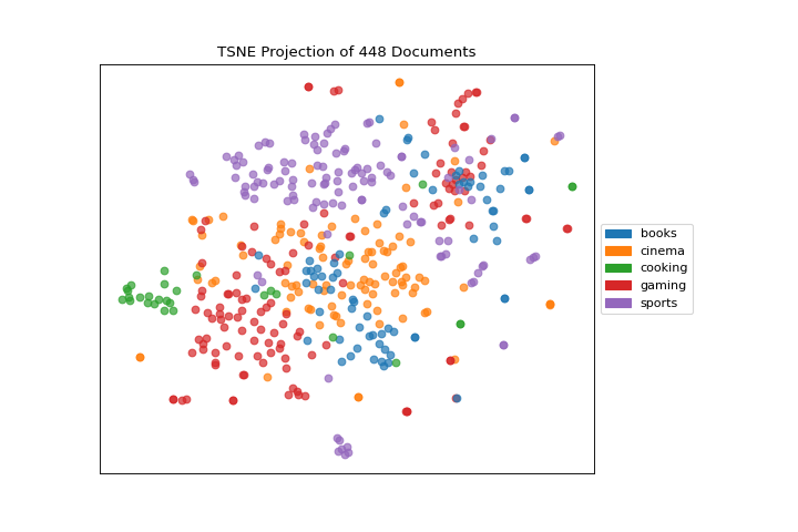
After importing the required tools, we can use the hobbies corpus and vectorize the text using TF-IDF. Once the corpus is vectorized we can visualize it, showing the distribution of classes.
from sklearn.feature_extraction.text import TfidfVectorizer

from yellowbrick.text import TSNEVisualizer
from yellowbrick.datasets import load_hobbies

# Load the data and create document vectors
corpus = load_hobbies()
tfidf = TfidfVectorizer()

X = tfidf.fit_transform(corpus.data)
y = corpus.target

# Create the visualizer and draw the vectors
tsne = TSNEVisualizer()
tsne.fit(X, y)
tsne.show()
(Source code, png, pdf)
Note that you can pass the class labels or document categories directly to the TSNEVisualizer as follows:
labels = corpus.labels
tsne = TSNEVisualizer(labels=labels)
tsne.fit(X, y)
tsne.show()
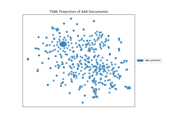
If we omit the target during fit, we can visualize the whole dataset to see if any meaningful patterns are observed.
(Source code, png, pdf)
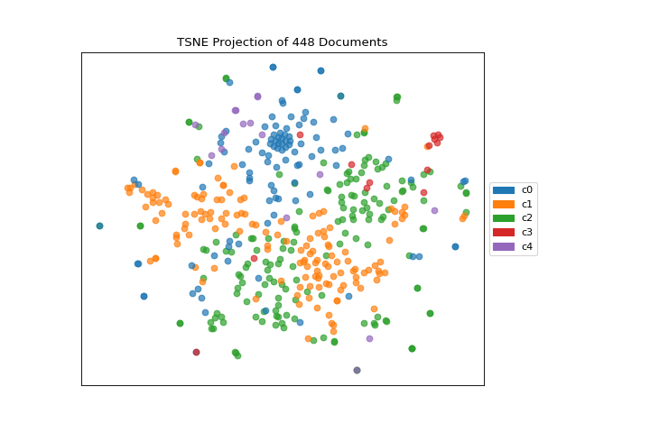
This means we don’t have to use class labels at all. Instead we can use cluster membership from K-Means to label each document. This will allow us to look for clusters of related text by their contents:
(Source code, png, pdf)
Quick Method
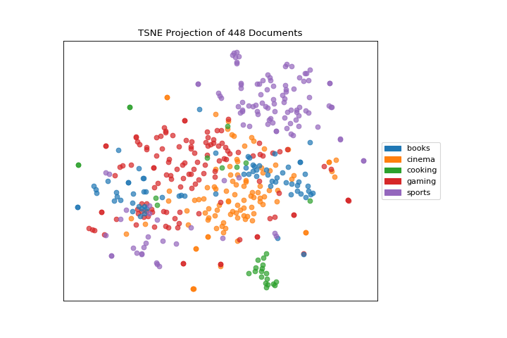
The same functionality above can be achieved with the associated quick method tsne. This method will build the TSNEVisualizer object with the associated arguments, fit it, then (optionally) immediately show it
from yellowbrick.text.tsne import tsne
from sklearn.feature_extraction.text import TfidfVectorizer
from yellowbrick.datasets import load_hobbies

# Load the data and create document vectors
corpus = load_hobbies()
tfidf = TfidfVectorizer()

X = tfidf.fit_transform(corpus.data)
y = corpus.target

tsne(X, y)
(Source code, png, pdf)

API Reference
Implements TSNE visualizations of documents in 2D space.
- class yellowbrick.text.tsne.TSNEVisualizer(ax=None, decompose='svd', decompose_by=50, labels=None, classes=None, colors=None, colormap=None, random_state=None, alpha=0.7, **kwargs)[source]
Bases:
TextVisualizerDisplay a projection of a vectorized corpus in two dimensions using TSNE, a nonlinear dimensionality reduction method that is particularly well suited to embedding in two or three dimensions for visualization as a scatter plot. TSNE is widely used in text analysis to show clusters or groups of documents or utterances and their relative proximities.
TSNE will return a scatter plot of the vectorized corpus, such that each point represents a document or utterance. The distance between two points in the visual space is embedded using the probability distribution of pairwise similarities in the higher dimensionality; thus TSNE shows clusters of similar documents and the relationships between groups of documents as a scatter plot.
TSNE can be used with either clustering or classification; by specifying the
classesargument, points will be colored based on their similar traits. For example, by passingcluster.labels_asyinfit(), all points in the same cluster will be grouped together. This extends the neighbor embedding with more information about similarity, and can allow better interpretation of both clusters and classes.For more, see https://lvdmaaten.github.io/tsne/
- Parameters
- axmatplotlib axes
The axes to plot the figure on.
- decomposestring or None, default:
'svd' A preliminary decomposition is often used prior to TSNE to make the projection faster. Specify
"svd"for sparse data or"pca"for dense data. If None, the original data set will be used.- decompose_byint, default: 50
Specify the number of components for preliminary decomposition, by default this is 50; the more components, the slower TSNE will be.
- labelslist of strings
The names of the classes in the target, used to create a legend. Labels must match names of classes in sorted order.
- colorslist or tuple of colors
Specify the colors for each individual class
- colormapstring or matplotlib cmap
Sequential colormap for continuous target
- random_stateint, RandomState instance or None, optional, default: None
If int, random_state is the seed used by the random number generator; If RandomState instance, random_state is the random number generator; If None, the random number generator is the RandomState instance used by np.random. The random state is applied to the preliminary decomposition as well as tSNE.
- alphafloat, default: 0.7
Specify a transparency where 1 is completely opaque and 0 is completely transparent. This property makes densely clustered points more visible.
- kwargsdict
Pass any additional keyword arguments to the TSNE transformer.
- NULL_CLASS = None
- draw(points, target=None, **kwargs)[source]
Called from the fit method, this method draws the TSNE scatter plot, from a set of decomposed points in 2 dimensions. This method also accepts a third dimension, target, which is used to specify the colors of each of the points. If the target is not specified, then the points are plotted as a single cloud to show similar documents.
- finalize(**kwargs)[source]
Finalize the drawing by adding a title and legend, and removing the axes objects that do not convey information about TNSE.
- fit(X, y=None, **kwargs)[source]
The fit method is the primary drawing input for the TSNE projection since the visualization requires both X and an optional y value. The fit method expects an array of numeric vectors, so text documents must be vectorized before passing them to this method.
- Parameters
- Xndarray or DataFrame of shape n x m
A matrix of n instances with m features representing the corpus of vectorized documents to visualize with tsne.
- yndarray or Series of length n
An optional array or series of target or class values for instances. If this is specified, then the points will be colored according to their class. Often cluster labels are passed in to color the documents in cluster space, so this method is used both for classification and clustering methods.
- kwargsdict
Pass generic arguments to the drawing method
- Returns
- selfinstance
Returns the instance of the transformer/visualizer
- make_transformer(decompose='svd', decompose_by=50, tsne_kwargs={})[source]
Creates an internal transformer pipeline to project the data set into 2D space using TSNE, applying an pre-decomposition technique ahead of embedding if necessary. This method will reset the transformer on the class, and can be used to explore different decompositions.
- Parameters
- decomposestring or None, default:
'svd' A preliminary decomposition is often used prior to TSNE to make the projection faster. Specify
"svd"for sparse data or"pca"for dense data. If decompose is None, the original data set will be used.- decompose_byint, default: 50
Specify the number of components for preliminary decomposition, by default this is 50; the more components, the slower TSNE will be.
- decomposestring or None, default:
- Returns
- transformerPipeline
Pipelined transformer for TSNE projections
- yellowbrick.text.tsne.tsne(X, y=None, ax=None, decompose='svd', decompose_by=50, labels=None, colors=None, colormap=None, alpha=0.7, show=True, **kwargs)[source]
Display a projection of a vectorized corpus in two dimensions using TSNE, a nonlinear dimensionality reduction method that is particularly well suited to embedding in two or three dimensions for visualization as a scatter plot. TSNE is widely used in text analysis to show clusters or groups of documents or utterances and their relative proximities.
- Parameters
- Xndarray or DataFrame of shape n x m
A matrix of n instances with m features representing the corpus of vectorized documents to visualize with tsne.
- yndarray or Series of length n
An optional array or series of target or class values for instances. If this is specified, then the points will be colored according to their class. Often cluster labels are passed in to color the documents in cluster space, so this method is used both for classification and clustering methods.
- axmatplotlib axes
The axes to plot the figure on.
- decomposestring or None
A preliminary decomposition is often used prior to TSNE to make the projection faster. Specify “svd” for sparse data or “pca” for dense data. If decompose is None, the original data set will be used.
- decompose_byint
Specify the number of components for preliminary decomposition, by default this is 50; the more components, the slower TSNE will be.
- labelslist of strings
The names of the classes in the target, used to create a legend.
- colorslist or tuple of colors
Specify the colors for each individual class
- colormapstring or matplotlib cmap
Sequential colormap for continuous target
- alphafloat, default: 0.7
Specify a transparency where 1 is completely opaque and 0 is completely transparent. This property makes densely clustered points more visible.
- showbool, default: True
If True, calls
show(), which in turn callsplt.show()however you cannot callplt.savefigfrom this signature, norclear_figure. If False, simply callsfinalize()- kwargsdict
Pass any additional keyword arguments to the TSNE transformer.
- Returns
- visualizer: TSNEVisualizer
Returns the fitted, finalized visualizer