Elbow Method

The KElbowVisualizer implements the “elbow” method to help data scientists select the optimal number of clusters by fitting the model with a range of values for \(K\). If the line chart resembles an arm, then the “elbow” (the point of inflection on the curve) is a good indication that the underlying model fits best at that point. In the visualizer “elbow” will be annotated with a dashed line.

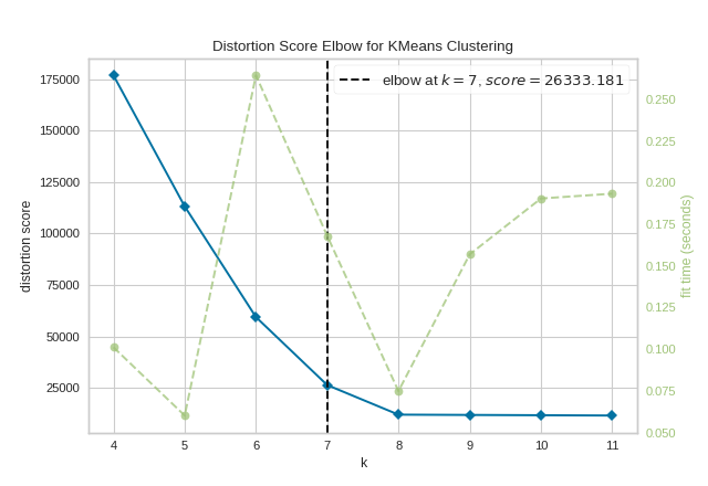
To demonstrate, in the following example the KElbowVisualizer fits the KMeans model for a range of \(K\) values from 4 to 11 on a sample two-dimensional dataset with 8 random clusters of points. When the model is fit with 8 clusters, we can see a line annotating the “elbow” in the graph, which in this case we know to be the optimal number.

Visualizer	KElbowVisualizer
Quick Method	kelbow_visualizer()
Models	Clustering
Workflow	Model evaluation

from sklearn.cluster import KMeans
from sklearn.datasets import make_blobs

from yellowbrick.cluster import KElbowVisualizer

# Generate synthetic dataset with 8 random clusters
X, y = make_blobs(n_samples=1000, n_features=12, centers=8, random_state=42)

# Instantiate the clustering model and visualizer
model = KMeans()
visualizer = KElbowVisualizer(model, k=(4,12))

visualizer.fit(X)        # Fit the data to the visualizer
visualizer.show()        # Finalize and render the figure

(Source code, png, pdf)

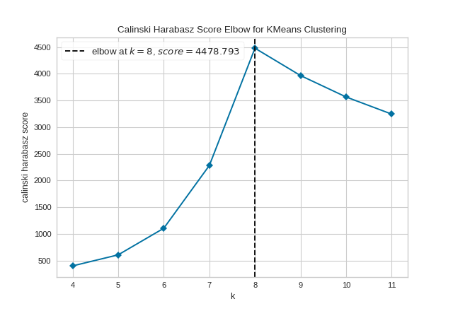
By default, the scoring parameter metric is set to distortion, which computes the sum of squared distances from each point to its assigned center. However, two other metrics can also be used with the KElbowVisualizer – silhouette and calinski_harabasz. The silhouette score calculates the mean Silhouette Coefficient of all samples, while the calinski_harabasz score computes the ratio of dispersion between and within clusters.

The KElbowVisualizer also displays the amount of time to train the clustering model per \(K\) as a dashed green line, but is can be hidden by setting timings=False. In the following example, we’ll use the calinski_harabasz score and hide the time to fit the model.

from sklearn.cluster import KMeans
from sklearn.datasets import make_blobs

from yellowbrick.cluster import KElbowVisualizer

# Generate synthetic dataset with 8 random clusters
X, y = make_blobs(n_samples=1000, n_features=12, centers=8, random_state=42)

# Instantiate the clustering model and visualizer
model = KMeans()
visualizer = KElbowVisualizer(
    model, k=(4,12), metric='calinski_harabasz', timings=False
)

visualizer.fit(X)        # Fit the data to the visualizer
visualizer.show()        # Finalize and render the figure

(Source code, png, pdf)

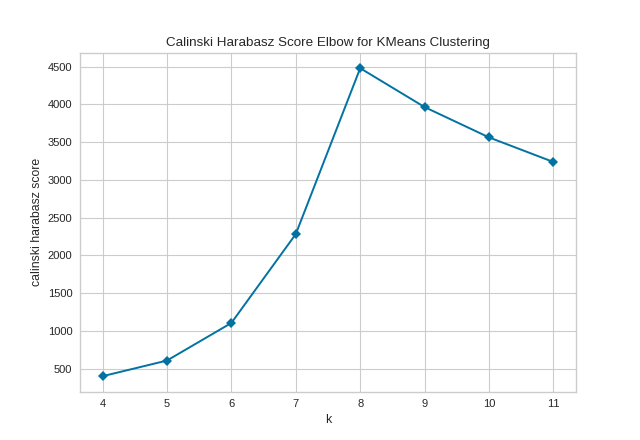
By default, the parameter locate_elbow is set to True, which automatically find the “elbow” which likely corresponds to the optimal value of k using the “knee point detection algorithm”. However, users can turn off the feature by setting locate_elbow=False. You can read about the implementation of this algorithm at “Knee point detection in Python” by Kevin Arvai.

In the following example, we’ll use the calinski_harabasz score and turn off locate_elbow feature.

from sklearn.cluster import KMeans
from sklearn.datasets import make_blobs

from yellowbrick.cluster import KElbowVisualizer

# Generate synthetic dataset with 8 random clusters
X, y = make_blobs(n_samples=1000, n_features=12, centers=8, random_state=42)

# Instantiate the clustering model and visualizer
model = KMeans()
visualizer = KElbowVisualizer(
    model, k=(4,12), metric='calinski_harabasz', timings=False, locate_elbow=False
)

visualizer.fit(X)        # Fit the data to the visualizer
visualizer.show()        # Finalize and render the figure

(Source code, png, pdf)

It is important to remember that the “elbow” method does not work well if the data is not very clustered. In this case, you might see a smooth curve and the optimal value of \(K\) will be unclear.

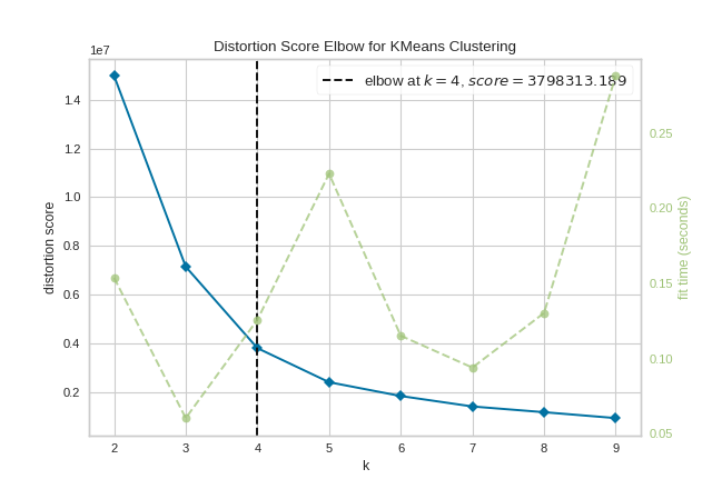
Quick Method

The same functionality above can be achieved with the associated quick method kelbow_visualizer. This method will build the KElbowVisualizer object with the associated arguments, fit it, then (optionally) immediately show the visualization.

from sklearn.cluster import KMeans
from yellowbrick.cluster.elbow import kelbow_visualizer
from yellowbrick.datasets.loaders import load_nfl

X, y = load_nfl()

# Use the quick method and immediately show the figure
kelbow_visualizer(KMeans(random_state=4), X, k=(2,10))

(Source code, png, pdf)

API Reference

Implements the elbow method for determining the optimal number of clusters. https://bl.ocks.org/rpgove/0060ff3b656618e9136b

class yellowbrick.cluster.elbow.KElbowVisualizer(estimator, ax=None, k=10, metric='distortion', distance_metric='euclidean', timings=True, locate_elbow=True, **kwargs)

Bases: ClusteringScoreVisualizer

The K-Elbow Visualizer implements the “elbow” method of selecting the optimal number of clusters for K-means clustering. K-means is a simple unsupervised machine learning algorithm that groups data into a specified number (k) of clusters. Because the user must specify in advance what k to choose, the algorithm is somewhat naive – it assigns all members to k clusters even if that is not the right k for the dataset.

The elbow method runs k-means clustering on the dataset for a range of values for k (say from 1-10) and then for each value of k computes an average score for all clusters. By default, the distortion score is computed, the sum of square distances from each point to its assigned center. Other metrics can also be used such as the silhouette score, the mean silhouette coefficient for all samples or the calinski_harabasz score, which computes the ratio of dispersion between and within clusters.

When these overall metrics for each model are plotted, it is possible to visually determine the best value for k. If the line chart looks like an arm, then the “elbow” (the point of inflection on the curve) is the best value of k. The “arm” can be either up or down, but if there is a strong inflection point, it is a good indication that the underlying model fits best at that point.

Parameters

estimatora scikit-learn clusterer

Should be an instance of an unfitted clusterer, specifically KMeans or MiniBatchKMeans. If it is not a clusterer, an exception is raised.

axmatplotlib Axes, default: None

The axes to plot the figure on. If None is passed in the current axes will be used (or generated if required).

kinteger, tuple, or iterable

The k values to compute silhouette scores for. If a single integer is specified, then will compute the range (2,k). If a tuple of 2 integers is specified, then k will be in np.arange(k[0], k[1]). Otherwise, specify an iterable of integers to use as values for k.

metricstring, default: "distortion"

Select the scoring metric to evaluate the clusters. The default is the mean distortion, defined by the sum of squared distances between each observation and its closest centroid. Other metrics include:

• distortion: mean sum of squared distances to centers

• silhouette: mean ratio of intra-cluster and nearest-cluster distance

• calinski_harabasz: ratio of within to between cluster dispersion

distance_metricstr or callable, default=’euclidean’

The metric to use when calculating distance between instances in a feature array. If metric is a string, it must be one of the options allowed by sklearn’s metrics.pairwise.pairwise_distances. If X is the distance array itself, use metric=”precomputed”.

timingsbool, default: True

Display the fitting time per k to evaluate the amount of time required to train the clustering model.

locate_elbowbool, default: True

Automatically find the “elbow” or “knee” which likely corresponds to the optimal value of k using the “knee point detection algorithm”. The knee point detection algorithm finds the point of maximum curvature, which in a well-behaved clustering problem also represents the pivot of the elbow curve. The point is labeled with a dashed line and annotated with the score and k values.

kwargsdict

Keyword arguments that are passed to the base class and may influence the visualization as defined in other Visualizers.

Notes

If you get a visualizer that doesn’t have an elbow or inflection point, then this method may not be working. The elbow method does not work well if the data is not very clustered; in this case, you might see a smooth curve and the value of k is unclear. Other scoring methods, such as BIC or SSE, also can be used to explore if clustering is a correct choice.

For a discussion on the Elbow method, read more at Robert Gove’s Block website. For more on the knee point detection algorithm see the paper “Finding a “kneedle” in a Haystack”.

See also

The scikit-learn documentation for the silhouette_score and calinski_harabasz_score. The default, distortion_score, is implemented in yellowbrick.cluster.elbow.

Examples

>>> from yellowbrick.cluster import KElbowVisualizer
>>> from sklearn.cluster import KMeans
>>> model = KElbowVisualizer(KMeans(), k=10)
>>> model.fit(X)
>>> model.show()

Attributes

k_scores_array of shape (n,) where n is no. of k values

The silhouette score corresponding to each k value.

k_timers_array of shape (n,) where n is no. of k values

The time taken to fit n KMeans model corresponding to each k value.

elbow_value_integer

The optimal value of k.

elbow_score_float

The silhouette score corresponding to the optimal value of k.

draw()

Draw the elbow curve for the specified scores and values of K.

finalize()

Prepare the figure for rendering by setting the title as well as the X and Y axis labels and adding the legend.

fit(X, y=None, **kwargs)

Fits n KMeans models where n is the length of self.k_values_, storing the silhouette scores in the self.k_scores_ attribute. The “elbow” and silhouette score corresponding to it are stored in self.elbow_value and self.elbow_score respectively. This method finishes up by calling draw to create the plot.

property metric_color

property timing_color

property vline_color

yellowbrick.cluster.elbow.kelbow_visualizer(model, X, y=None, ax=None, k=10, metric='distortion', distance_metric='euclidean', timings=True, locate_elbow=True, show=True, **kwargs)

Quick Method:

modela Scikit-Learn clusterer

Should be an instance of an unfitted clusterer, specifically KMeans or MiniBatchKMeans. If it is not a clusterer, an exception is raised.

Xarray-like of shape (n, m)

A matrix or data frame with n instances and m features

yarray-like of shape (n,), optional

A vector or series representing the target for each instance

axmatplotlib Axes, default: None

The axes to plot the figure on. If None is passed in the current axes will be used (or generated if required).

kinteger, tuple, or iterable

The k values to compute silhouette scores for. If a single integer is specified, then will compute the range (2,k). If a tuple of 2 integers is specified, then k will be in np.arange(k[0], k[1]). Otherwise, specify an iterable of integers to use as values for k.

metricstring, default: "distortion"

Select the scoring metric to evaluate the clusters. The default is the mean distortion, defined by the sum of squared distances between each observation and its closest centroid. Other metrics include:

• distortion: mean sum of squared distances to centers

• silhouette: mean ratio of intra-cluster and nearest-cluster

  distance

• calinski_harabasz: ratio of within to between cluster dispersion

distance_metricstr or callable, default=’euclidean’

The metric to use when calculating distance between instances in a feature array. If metric is a string, it must be one of the options allowed by sklearn’s metrics.pairwise.pairwise_distances. If X is the distance array itself, use metric=”precomputed”.

timingsbool, default: True

Display the fitting time per k to evaluate the amount of time required to train the clustering model.

locate_elbowbool, default: True

Automatically find the “elbow” or “knee” which likely corresponds to the optimal value of k using the “knee point detection algorithm”. The knee point detection algorithm finds the point of maximum curvature, which in a well-behaved clustering problem also represents the pivot of the elbow curve. The point is labeled with a dashed line and annotated with the score and k values.

showbool, default: True

If True, calls show(), which in turn calls plt.show() however you cannot call plt.savefig from this signature, nor clear_figure. If False, simply calls finalize()

kwargsdict

Keyword arguments that are passed to the base class and may influence the visualization as defined in other Visualizers.

Returns

vizKElbowVisualizer

The kelbow visualizer, fitted and finalized.