Cook’s Distance

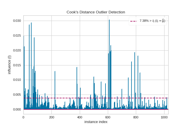
Cook’s Distance is a measure of an observation or instances’ influence on a linear regression. Instances with a large influence may be outliers, and datasets with a large number of highly influential points might not be suitable for linear regression without further processing such as outlier removal or imputation. The CooksDistance visualizer shows a stem plot of all instances by index and their associated distance score, along with a heuristic threshold to quickly show what percent of the dataset may be impacting OLS regression models.

Visualizer	`CooksDistance`
Quick Method	`cooks_distance()`
Models	General Linear Models
Workflow	Dataset/Sensitivity Analysis

from yellowbrick.regressor import CooksDistance
from yellowbrick.datasets import load_concrete

# Load the regression dataset
X, y = load_concrete()

# Instantiate and fit the visualizer
visualizer = CooksDistance()
visualizer.fit(X, y)
visualizer.show()

(Source code, png, pdf)

The presence of so many highly influential points suggests that linear regression may not be suitable for this dataset. One or more of the four assumptions behind linear regression might be being violated; namely one of: independence of observations, linearity of response, normality of residuals, or homogeneity of variance (“homoscedasticity”). We can check the latter three conditions using a residual plot:

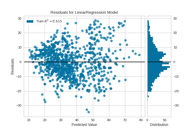
from sklearn.linear_model import LinearRegression
from yellowbrick.regressor import ResidualsPlot

# Instantiate and fit the visualizer
model = LinearRegression()
visualizer_residuals = ResidualsPlot(model)
visualizer_residuals.fit(X, y)
visualizer_residuals.show()

(Source code, png, pdf)

The residuals appear to be normally distributed around 0, satisfying the linearity and normality conditions. However, they do skew slightly positive for larger predicted values, and also appear to increase in magnitude as the predicted value increases, suggesting a violation of the homoscedasticity condition.

Given this information, we might consider one of the following options: (1) using a linear regression anyway, (2) using a linear regression after removing outliers, and (3) resorting to other regression models. For the sake of illustration, we will go with option (2) with the help of the Visualizer’s public learned parameters distance_ and influence_threshold_:

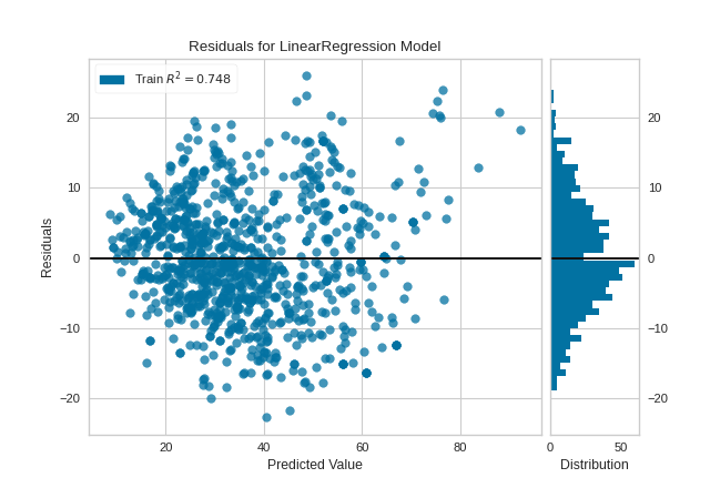
i_less_influential = (visualizer.distance_ <= visualizer.influence_threshold_)
X_li, y_li = X[i_less_influential], y[i_less_influential]

model = LinearRegression()
visualizer_residuals = ResidualsPlot(model)
visualizer_residuals.fit(X_li, y_li)
visualizer_residuals.show()

(Source code, png, pdf)

Residual plot using concrete dataset after outlier removal

The violations of the linear regression assumptions addressed earlier appear to be diminished. The goodness-of-fit measure has increased from 0.615 to 0.748, which is to be expected as there is less variance in the response variable after outlier removal.

Quick Method

Similar functionality as above can be achieved in one line using the associated quick method, cooks_distance. This method will instantiate and fit a CooksDistance visualizer on the training data, then will score it on the optionally provided test data (or the training data if it is not provided).

from yellowbrick.datasets import load_concrete
from yellowbrick.regressor import cooks_distance

# Load the regression dataset
X, y = load_concrete()

# Instantiate and fit the visualizer
cooks_distance(
    X, y,
    draw_threshold=True,
    linefmt="C0-", markerfmt=","
)

(Source code, png, pdf)

API Reference

Visualize the influence and leverage of individual instances on a regression model.

class yellowbrick.regressor.influence.CooksDistance(ax=None, draw_threshold=True, linefmt='C0-', markerfmt=',', **kwargs)[source]

Bases: Visualizer

Cook’s Distance is a measure of how influential an instance is to the computation of a regression, e.g. if the instance is removed would the estimated coeficients of the underlying model be substantially changed? Because of this, Cook’s Distance is generally used to detect outliers in standard, OLS regression. In fact, a general rule of thumb is that D(i) > 4/n is a good threshold for determining highly influential points as outliers and this visualizer can report the percentage of data that is above that threshold.

This implementation of Cook’s Distance assumes Ordinary Least Squares regression, and therefore embeds a sklearn.linear_model.LinearRegression under the hood. Distance is computed via the non-whitened leverage of the projection matrix, computed inside of fit(). The results of this visualizer are therefore similar to, but not as advanced, as a similar computation using statsmodels. Computing the influence for other regression models requires leave one out validation and can be expensive to compute.

See also

For a longer discussion on detecting outliers in regression and computing leverage and influence, see linear regression in python, outliers/leverage detect by Huiming Song.

Parameters

axmatplotlib Axes, default: None: The axes to plot the figure on. If None is passed in the current axes will be used (or generated if required).
draw_thresholdbool, default: True: Draw a horizontal line at D(i) == 4/n to easily identify the most influential points on the final regression. This will also draw a legend that specifies the percentage of data points that are above the threshold.
linefmtstr, default: ‘C0-’: A string defining the properties of the vertical lines of the stem plot, usually this will be a color or a color and a line style. The default is simply a solid line with the first color of the color cycle.
markerfmtstr, default: ‘,’: A string defining the properties of the markers at the stem plot heads. The default is “pixel”, e.g. basically no marker head at the top of the stem plot.
kwargsdict: Keyword arguments that are passed to the base class and may influence the final visualization (e.g. size or title parameters).

Notes

Cook’s Distance is very similar to DFFITS, another diagnostic that is meant to show how influential a point is in a statistical regression. Although the computed values of Cook’s and DFFITS are different, they are conceptually identical and there even exists a closed-form formula to convert one value to another. Because of this, we have chosen to implement Cook’s distance rather than or in addition to DFFITS.

Attributes

distance_array, 1D: The Cook’s distance value for each instance specified in X, e.g. an 1D array with shape (X.shape[0],).
p_values_array, 1D: The p values associated with the F-test of Cook’s distance distribution. A 1D array whose shape matches distance_.
influence_threshold_float: A rule of thumb influence threshold to determine outliers in the regression model, defined as It=4/n.
outlier_percentage_float: The percentage of instances whose Cook’s distance is greater than the influnce threshold, the percentage is 0.0 <= p <= 100.0.

draw()[source]: Draws a stem plot where each stem is the Cook’s Distance of the instance at the index specified by the x axis. Optionaly draws a threshold line.

finalize()[source]: Prepares the visualization for presentation and reporting.

fit(X, y)[source]

Computes the leverage of X and uses the residuals of a sklearn.linear_model.LinearRegression to compute the Cook’s Distance of each observation in X, their p-values and the number of outliers defined by the number of observations supplied.

Parameters

Xarray-like, 2D: The exogenous design matrix, e.g. training data.
yarray-like, 1D: The endogenous response variable, e.g. target data.

Returns

selfCooksDistance: Fit returns the visualizer instance.

yellowbrick.regressor.influence.cooks_distance(X, y, ax=None, draw_threshold=True, linefmt='C0-', markerfmt=',', show=True, **kwargs)[source]

Cook’s Distance is a measure of how influential an instance is to the computation of a regression, e.g. if the instance is removed would the estimated coeficients of the underlying model be substantially changed? Because of this, Cook’s Distance is generally used to detect outliers in standard, OLS regression. In fact, a general rule of thumb is that D(i) > 4/n is a good threshold for determining highly influential points as outliers and this visualizer can report the percentage of data that is above that threshold.

This implementation of Cook’s Distance assumes Ordinary Least Squares regression, and therefore embeds a sklearn.linear_model.LinearRegression under the hood. Distance is computed via the non-whitened leverage of the projection matrix, computed inside of fit(). The results of this visualizer are therefore similar to, but not as advanced, as a similar computation using statsmodels. Computing the influence for other regression models requires leave one out validation and can be expensive to compute.